Longitudinal Shear Stress Concentration Produced by a Long Straight Opening in an Elastic Mass

R.G. Friday

Summary.—The stress concentration factors relating three dimensional field stress to stresses at the boundary of a long straight opening of uniform cross-section, may be readily determined except for those relating longitudinal shear stresses. A theory developed in this paper leads to the principle that longitudinal shear stress at any point is given by modulus of rigidity times the gradient of longitudinal displacement ( $w$ ), where $w$ satisfies Laplace’s equation in the region outside the opening and the necessary boundary conditions. A method of solution by conformal mapping is outlined and results for certain openings are tabulated.

List of Symbols

$x,y,z$	Reference axes (see Fig. 1 (a)).
$n$	Normal	axes at a point on opening boundary.
$t$	Tangential
$l$	Longitudinal
$\sigma$	Direct stress	Subscript $F$ applies to stresses remote from opening.
$\tau$	Shear stress	Subscript $F$ applies to stresses remote from opening.
$\nu$	Poisson’s ratio.
$G$	Modulus of rigidity
$a_x, a_{xy}, etc$	Stress Concentration factors
$u,v,w$	Displacements in $x,y,z$ directions.
$\varepsilon$	Direct strain.
$\gamma$	Shear strain.
$r, \theta$	Polar co-ordinates (see Fig. 2).
$a$	Radius of a circular opening.
$Z = x + iy$	Complex variable.
$\xi = \alpha \ cis \ \beta$	Complex variable.
$A, B, C —$	Transformation coefficients.
$m, N$	Integers.

1.—INTRODUCTION

In designing an underground opening it is generally required to estimate the stresses in the rock close to the excavation boundary. This paper is concerned with the relation between the three-dimensional field stress and the stresses around a long straight opening of uniform cross-section. This relation must also be known to calculate virgin stresses from stress measurements taken at a tunnel boundary.

It is assumed that the opening occurs in a homogeneous, isotropic elastic mass of material which, away from the disturbing influence of the opening, is uniformly stressed. The stress distribution around the opening . is the same whether the opening is cut before stress application, as in many engineering structures, or after stress application as for excavations in rock.

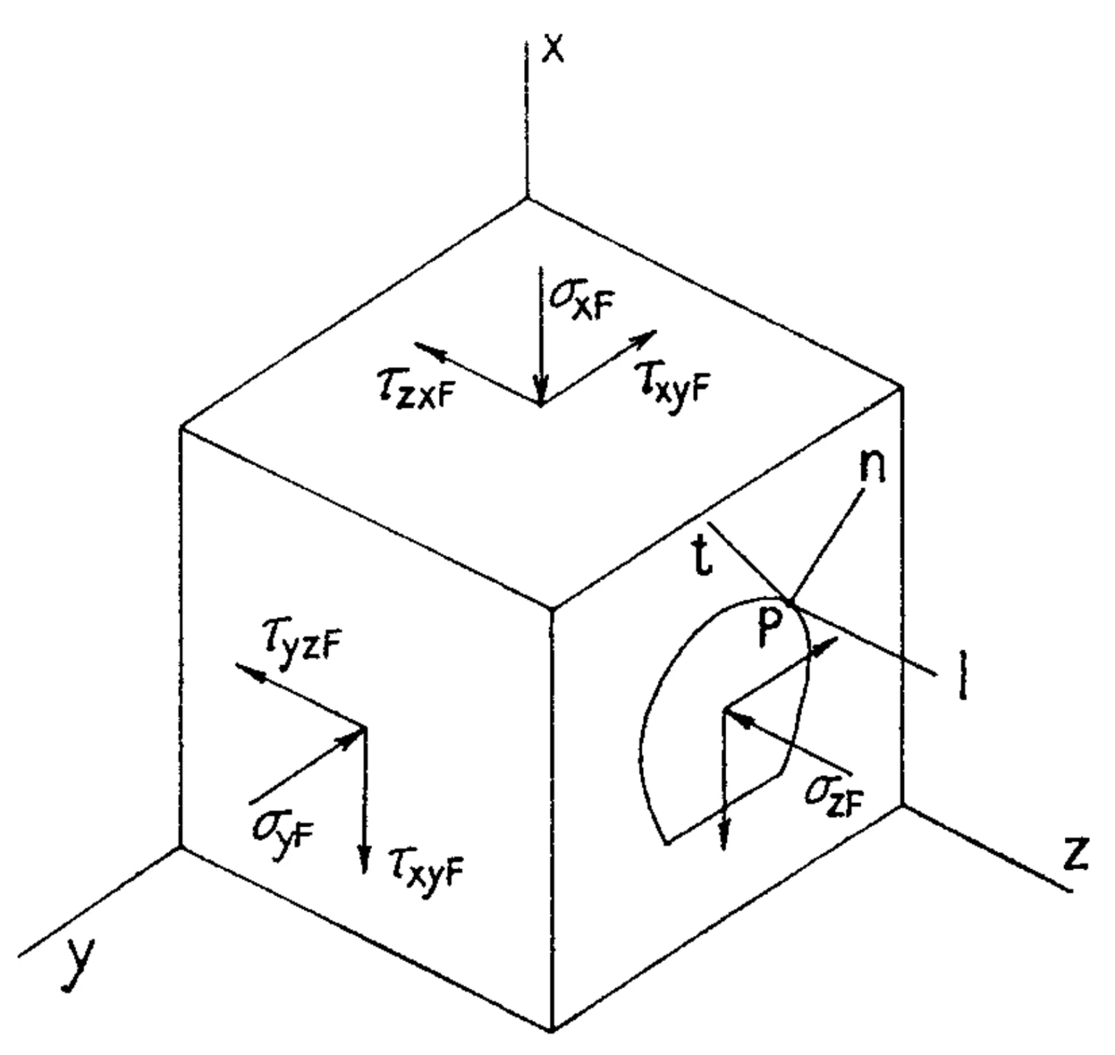
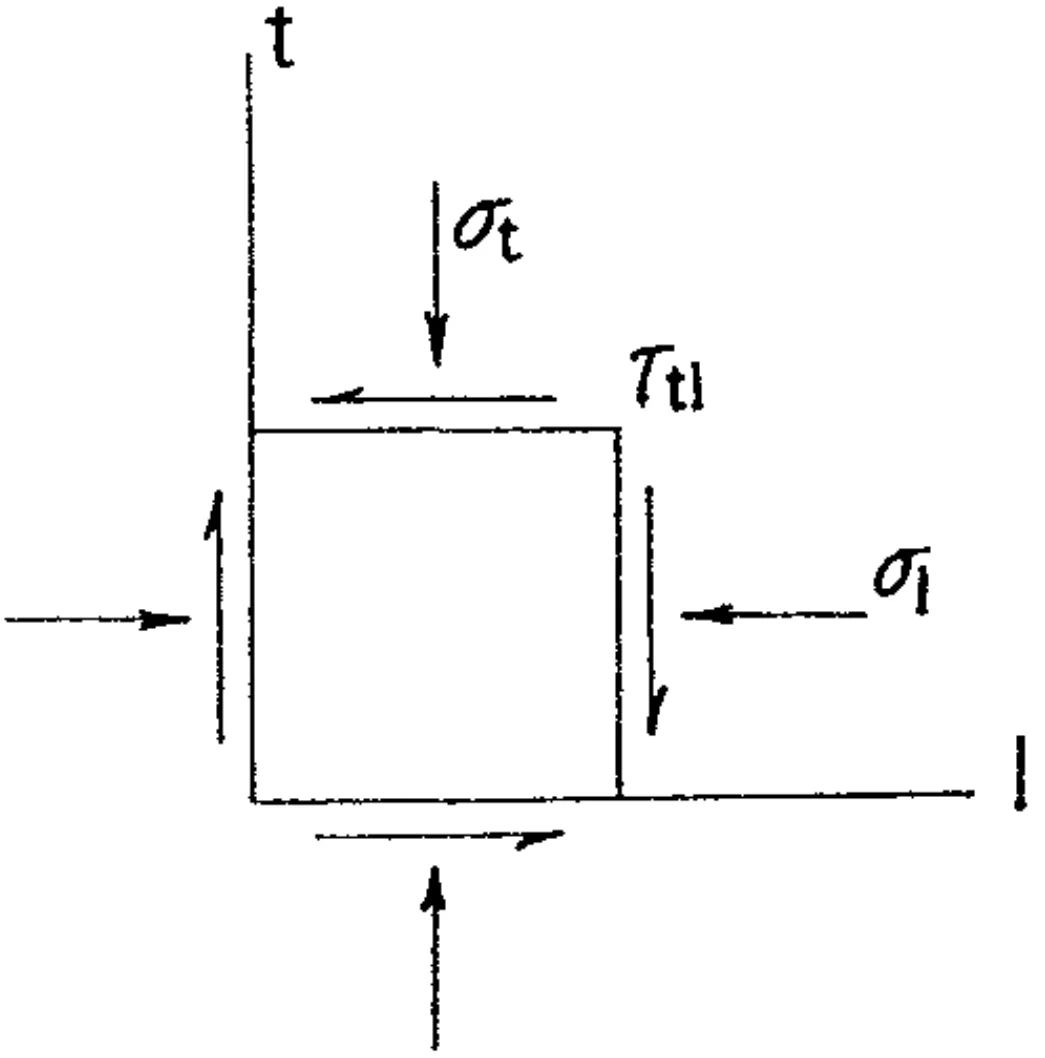
Fig. 1 (a) shows the six components of the virgin stress field and the opening with its axis in the $z$ -direction. The $x$ -axis has been directed vertically for convenience in analysis later. Fig. 1 (b) shows the three stress components at a point $P$ on the opening boundary. These three components may be expressed in terms of the field stress components thus:

\begin{equation} \sigma _t = a_x \ \sigma _{xF} + a_y \ \sigma _{yF} + a_{xy} \ \tau _{xyF} \label{eq:1} \end{equation} \ref{eq:1} (1)

\begin{equation} \sigma _l = \sigma _{zF} + \nu(a_x – 1) \ \sigma _{xF} + \nu (a_y – 1) \ \sigma _{yF} + \nu a _{xy} \ \tau _{xyF} \label{eq:2} \end{equation} \ref{eq:2} (2)

\begin{equation} \tau _{tl} = a _{yz} \ \tau _{yzF} + a_{zx} \ \tau _{zxF} \label{eq:3} \end{equation} \ref{eq:3} (3)

in which the $a$ ‘s are stress concentration factors applying at the point $P$ considered. These three equations were given by Hiramatsu and Oka (Ref. 1). The stresses $\sigma_{xF}$ , $\sigma_{yF}$ and $\tau _{xyF}$ appear in Eq. (2) to satisfy the condition that excavation of the opening produces no change in longitudinal strain.

The stress concentration factors $a_x$ , $a_y$ and $a_{xy}$ may be determined readily by two-dimensional photoelastic models (Ref. 2) or by mathematical methods (Ref. 3).

The author could find no reference giving a general solution for determining the longitudinal shear stress concentration factors $a_{yz}$ and $a_{zx}$ . Ref. 6, Ref. 1 and others provide theoretical results for the region around a circular opening. Hiramatsu and Oka (Ref. 1) determined values of $a_{yz}$ and $a_{zx}$ for certain openings by three-dimensional photo-elastic experiments. However, the technique is rather specialized and the results obtained for a circular opening did not agree well with the theoretical ones.

Fig. 1 (a).—Opening in Three-Dimensional Stress Field.

Fig. 1 (b).—Stresses at a Point on the Opening Boundary.

2.—THEORY FOR LONGITUDINAL SHEAR

The approach followed is similar to that in the Saint-Venant solution for torsion of prismatic bars (Ref. 4, p. 259).

The application of a field longitudinal shear stress such as $\tau _{yzF}$ or $\tau _{zxF}$ will produce warping of planes perpendicular to the opening axis ( $z$ -axis).

w = w(x,y)

Since the cross-section is uniform there will be no change with respect to $z$ . Therefore

No displacement perpendicular to the $z$ -axis can occur. For example, if the application of $\tau _{zxF}$ were to produce a displacement $u = k \tau _{zxF}$ at a point, then the application of — $\tau _{zxF}$ would have to produce a displacement $u = – k \tau _{zxF}$ at the same point. Such behaviour is inconceivable in the model considered. Therefore

\begin{equation} u = \nu = 0 \label{eq:5} \end{equation} \ref{eq:5} (5)

Because of Eqs. (4) and (5),

\therefore \begin{array}{l l} & \epsilon _x = \epsilon _y = \epsilon _z = \gamma _{xy} = 0 \\ & \sigma _x = \sigma _y = \sigma _z = \tau _{xy} = 0 \label{eq:6} \end{array} \ref{eq:6} (6)

But

\tau _{yz} = G \ \gamma _{yz} = G \left( \frac{\partial v}{\partial z} + \frac{\partial w}{\partial y} \right)

and since $\nu = 0$

\begin{equation} \tau _{yz} = G \frac{\partial w}{\partial y} \label{eq:7} \end{equation} \ref{eq:7} (7)

\begin{equation} \tau _{zx} = G \frac{\partial w}{\partial x} \label{eq:8} \end{equation} \ref{eq:8} (8)

For equilibrium, since $\sigma _z$ does not vary with $z$

\begin{equation} \frac{\partial \tau _{yz}}{\partial y} + \frac{\partial \tau _{zx}}{\partial x} = 0 \label{eq:9} \end{equation} \ref{eq:9} (Ref. 4, p. 229) (9)

Substituting Eqs. (7) and (8) gives

\begin{equation} \frac{\partial \tau _{yz}}{\partial y} + \frac{\partial ^2 w}{\partial x^2} = 0 \label{eq:10} \end{equation} \ref{eq:10} (10)

That is, the displacement parallel to the opening axis satisfies Laplace’s equation.

2.2 Boundary Conditions:

At the boundary of the opening

\begin{equation} \tau _{nt} = 0 \end{equation}

and

\begin{equation} \tau _{nl} = 0 \end{equation}

The first is already satisfied by Eq. (6). The second will be satisfied by putting

\begin{equation} \gamma _{nl} = \frac{\partial w}{\partial n} = 0 \label{eq:11} \end{equation} \ref{eq:11} (11)

at the opening boundary.

The conditions away from the influence of the opening are

\begin{array}{l} & \tau _{yz} = \tau _{yzF} \\ & \tau _{zx} = \tau _{zxF} \end{array}

Substituting Eqs. (7) and (8) gives the conditions remote from the opening:

\begin{equation} \begin{array}{} \frac{\partial w}{\partial y} = \frac{1}{G} \ \tau _{yzF} \\ \frac{\partial w}{\partial x} = \frac{1}{G} \ \tau _{zxF} \end{array} \label{eq:12} \end{equation} \ref{eq:12} (12)

2.3 Principle:

The magnitude of the longitudinal shear stress at any point is given by $G$ times the gradient of $w$ (longitudinal displacement) where $w$ satisfies Laplace’s equation (10) and the boundary conditions (11) and (12). The direction of the shear stress on the $x$ – $y$ plane is given by the direction of the gradient.

3.—METHODS OF SOLUTION

3.1 General:

The shear stress distribution around an opening of given cross-section could be determined by mathematical analysis, finite difference method or analogue methods.

An attempt was made to obtain solutions by measuring relative voltage gradients on a sheet of conducting paper with a hole cut at the centre to represent the opening shape. Consistent results were not obtained. The results below were obtained by mathematical analysis.

3.2 Circular Hole:

The solution for shear stress in the region around a circular hole in a mass under longitudinal shear stress is mathematically identical to that for ideal fluid flow past a circular cylinder (Ref. 5, p. 547) (see Fig. 2).

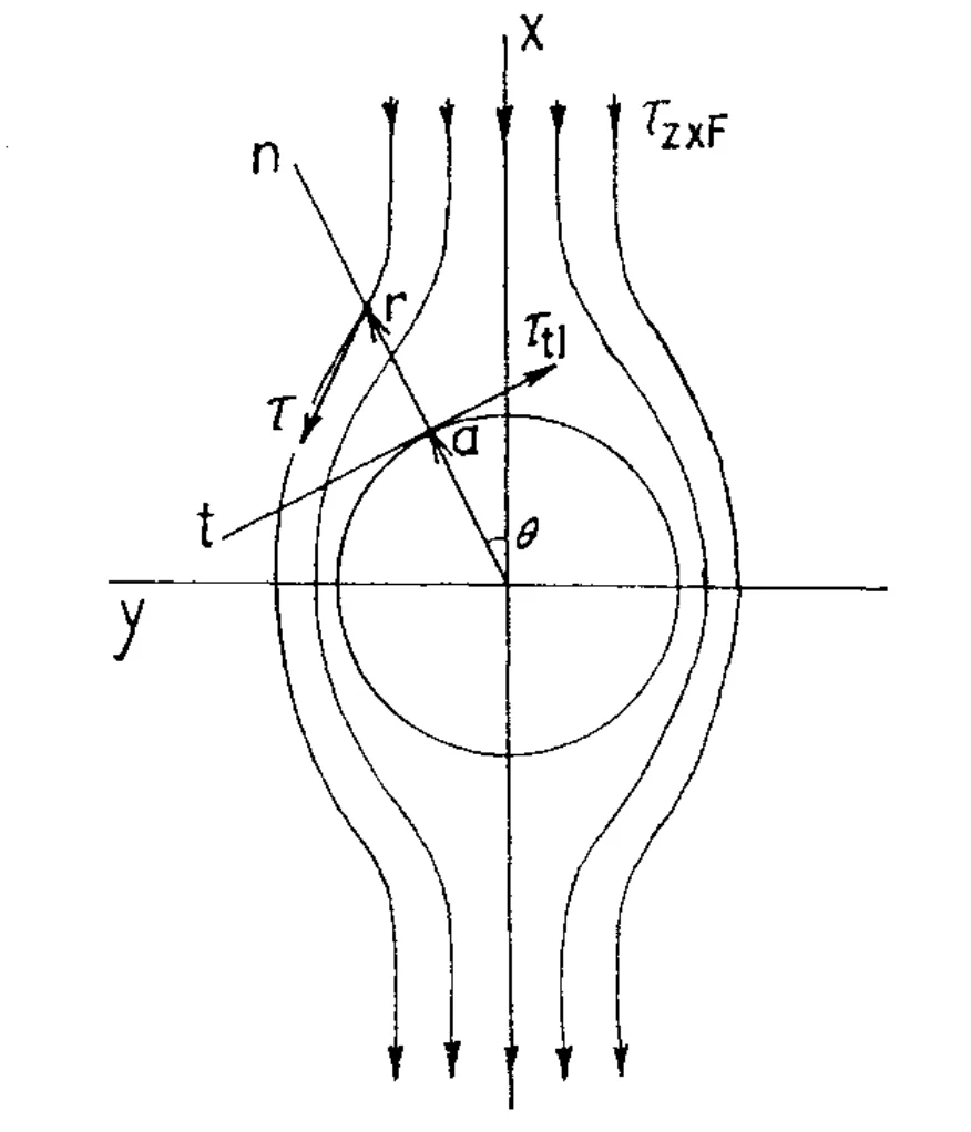
Fig. 2.-Longitudinal Shear Stress Distribution Around a Circular Opening.

For field stress $\tau _{zxF}$

\tau = \tau _{zxF} \sqrt{ 1 – 2 \left( \frac{a}{r} \right) ^2 \cos 2 \theta + \left( \frac{a}{r} \right) ^4 }

At the boundary $r = a$

\begin{equation} \tau _{tl} = -2 \ \gamma _{zxF} \ \sin \theta \label{eq:13} \end{equation} \ref{eq:13} (13)

This agrees with previous theoretical solutions (Ref. 1 and Ref. 6).

3.3 Openings of Other Shapes:

A single opening of any cross-section may, in principle, be dealt with by conformal mapping using transformations $Z= f(\zeta)$ of the form

\begin{equation} Z = A \zeta + \frac{B}{\zeta} + \frac{C}{\zeta ^2} + \frac{D}{\zeta ^3} + – – – + P \label{eq:14} \end{equation} \ref{eq:14} (14)

This produces a 1-to-1 transformation of points outside the unit circle on the $\zeta$ -plane to points outside a corresponding boundary on the $Z$ -plane.

If the transformation coefficients $A$ to $P$ are restricted to real values then only openings symmetrical about the $x$ -axis may be dealt with. This restriction is applied to simplify the work from here on.

An opening boundary on the $\zeta$ plane defined by the unit circle $\zeta = \cos \beta + \iota \sin \beta$ is transformed on the $Z$ -plane to an opening boundary defined by

\begin{equation} \begin{array}{} x = (A + B) \cos \beta + C \cos 2 \beta + D \cos 3 \beta + – – – + P \\ y = (A-B) \sin \beta – C \sin 2 \beta – D \sin 3 \beta – – – – \end{array} \label{eq:15} \end{equation} \ref{eq:15} (15)

where $Z = x + \iota y$

By choosing suitable values for the coefficients $A$ to $P$ the boundary on the $Z$ -plane may be made to approximate any shape having symmetry about the $x$ -axis.

Laplace’s equation is still satisfied after the transformation and by analogy with solutions for fluid flow (Ref. 5, p. 543) it is found that the magnitude of the shear stress at a point $Z_0$ on the $Z$ plane is obtained by dividing the magnitude of the shear stress at the corresponding point $\zeta _0$ on the $\zeta$ -plane by $| \sideset{}{‘} f (\zeta_0) |$ .

\begin{equation} \tau _{tlZ_0} = \tau _{tl \zeta_0} / | \sideset{}{‘} f (\zeta_0) | \label{eq:16} \end{equation} \ref{eq:16} (16)

Now for the transformation (14)

\begin{equation} \sideset{}{‘} f (\zeta) = A – \frac{B}{\zeta ^2} – \frac{2C}{\zeta ^3} – \frac{3D}{\zeta ^4} – \frac{4E}{\zeta ^5} – – – \end{equation}

For points on the opening boundary $\zeta = \cos \beta + \iota \sin \beta$ , the first five terms of (14) give

\begin{equation} \begin{array}{} | \sideset{}{‘} f (\zeta_0) | = \sqrt{ \left[ A^2 + B^2 + 4C^2 + 9D^2 + 16E^2 + 2 \cos \beta(2BC + 6CD + 12DE) + 2\cos 2\beta (-AB + 3BD + 8CE) + 2 \cos 3\beta (-2AC + 4BE) + 2 \cos 4 \beta (-3AD) + 2 \cos 5 \beta (-4AE) \right] } \end{array} \label{eq:17} \end{equation} \ref{eq:17} (17)

For points remote from the opening $| \sideset{}{‘} f (\zeta) |$ approaches $A$ . To obtain equality between the shear stresses remote from the opening on the $Z$ – and $\zeta$ -planes the factor $A$ is introduced to Eq. (16). Eq. (13) is re-written to refer to the $\zeta$ -plane:

\begin{equation} \tau _{tl \zeta_0} = -2 \tau _{zxF} \ \sin \beta \end{equation}

and substituted in Eq. (16). Then

\begin{equation} \tau _{tlZ_0} = – 2 \tau _{zxF} \ \sin \beta \ \frac{A}{| \sideset{}{‘} f (\zeta_0) |} \end{equation}

The shear stress concentration factor is then

\begin{equation} a_{zx} = \frac{\tau _{tlZ}}{\tau _{zxF}} = – \frac{2 \sin \beta A}{| \sideset{}{‘} f (\zeta_0) |} \label{eq:18} \end{equation} \ref{eq:18} (18)

where $| \sideset{}{‘} f (\zeta_0) |$ may be calculated from Eq. (17).

For field stress $\tau _{yzF}$ Eq. (13) becomes (see Fig. 2)

\begin{array}{c l} & \tau _{tl} = & – 2 \tau _{yzF} \sin \left( \theta – \frac{\pi}{2} \right) \\ & &= 2 \tau _{yzF} \ \cos \theta \end{array}

The shear stress concentration factor is then

\begin{equation} a_{yz} = \frac{\tau _{tlZ}}{\tau _{yzF}} = \frac{2 \ \cos \beta A}{| \sideset{}{‘} f (\zeta_0) |} \label{eq:19} \end{equation} \ref{eq:19} (19)

Transformation Coefficients and Longitudinal Shear Stress Concentration Factors for Various Openings

	Circle	2:1 Ellipse	Square	2:1 Rectangle	Horseshoe	Particular Tunnel
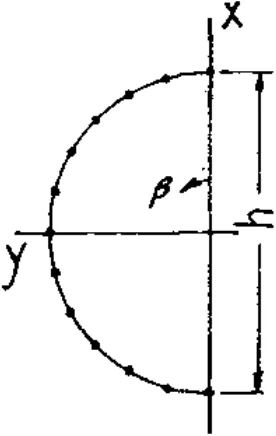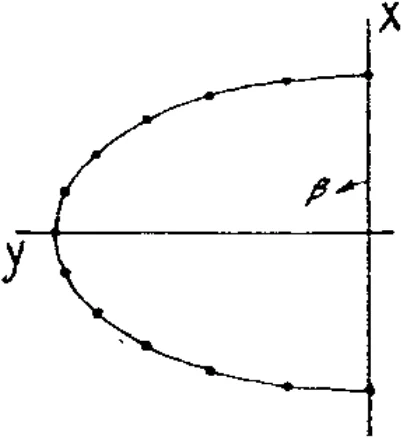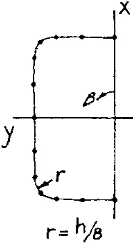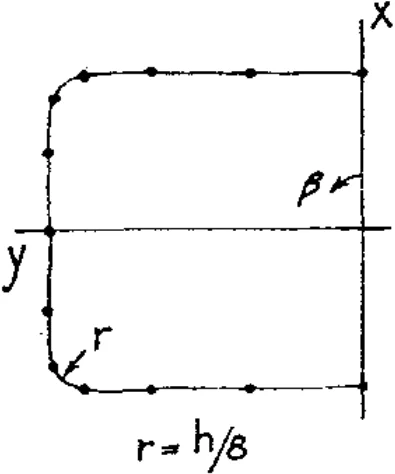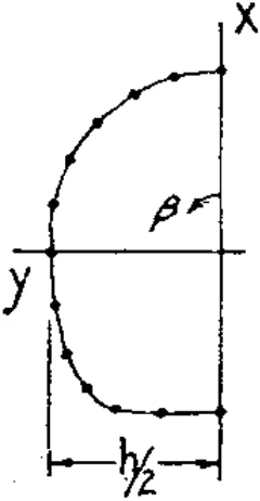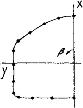A	0.5	0.75	0.5763	0.8639	0.5215	0.6586
B	0	-0.25	0.0000	-0.2652	0.0047	-0.1272
C	0	0	0.0000	0.0000	0.0170	0.0585
D	0	0	-0.0777	-0.1161	-0.0218	-0.0438
E	0	0	0.0000	0.0000	0.0137	0.0257
F	0	0	0.0000	0.0146	-0.0044	0.0159
G	0	0	0.0000	0.0000	0.0005	-0.0081
H	0	0	0.0013	0.0022	-0.0001	-0.0035
$\beta$	$a_{zx}$	$a_{yz}$	$a_{zx}$	$a_{yz}$	$a_{zx}$	$a_{yz}$	$a_{zx}$	$a_{yz}$	$a_{zx}$	$a_{yz}$	$a_{zx}$	$a_{yz}$
0	0.00	2.00	0.00	1.50	0.00	1.44	0.00	1.24	0.00	2.03	0.00	1.91
15	-0.52	1.93	-0.40	1.49	-0.41	1.54	-0.34	1.26	-0.53	1.97	-0.49	1.82
30	-1.00	1.73	-0.83	1.44	-1.13	1.96	-0.82	1.42	-1.01	1.76	-0.85	1.48
45	-1.41	1.41	-1.34	1.34	-2.44	2.44	-2.02	2.02	-1.42	1.42	-1.23	1.23
60	-1.73	1.00	-1.96	1.13	-1.96	1.13	-3.00	1.73	-1.74	1.01	-2.08	1.20
75	-1.93	0.52	-2.64	0.71	-1.54	0.41	-1.97	0.53	-1.89	0.51	-2.34	0.63
90	-2.00	0.00	-3.00	0.00	-1.44	0.00	-1.72	0.00	-1.83	0.00	-1.72	0.00
105	-1.93	-0.52	-2.64	-0.71	-1.54	-0.41	-1.97	-0.53	-1.72	-0.46	-1.82	-0.49
120	-1.73	-1.00	-1.96	-1.13	-1.96	-1.13	-3.00	-1.73	-1.74	-1.01	-3.12	-1.80
135	-1.41	-1.41	-1.34	-1.34	-2.44	-2.44	-2.02	-2.02	-1.85	-1.85	-2.12	-2.12
150	-1.00	-1.73	-0.83	-1.44	-1.13	-1.96	-0.82	-1.42	-1.21	-2.10	-0.84	-1.46
165	-0.52	-1.93	-0.40	-1.49	-0.41	-1.54	-0.34	-1.26	-0.44	-1.66	-0.35	-1.30
180	0.00	-2.00	0.00	-1.50	0.00	-1.44	0.00	-1.24	0.00	-1.50	0.00	-1.27

4.—COMPUTER PROGRAM

A computer program was developed to

determine the transformation coefficients for an opening boundary defined by x and y co-ordinates of up to 10 points above the x-axis and 2 points on the x-axis,
plot the resulting mathematical outline according to Eq. (15),
calculate shear stress concentration factors according to Eqs. (18) and (19) for a succession of points around the boundary.

Part (a) was based on the method followed in Ref. 3 and is outlined in the Appendix. The program was run on the CDC.6400 computer at the University of Adelaide.

5.—RESULTS

Table I shows transformation coefficients and longitudinal shear stress concentration factors for several opening shapes. All the openings are symmetrical about the x-axis.

It was found that 8 terms in the transformation Eq. (14) were sufficient to give a good approximation to the opening shapes considered. In the diagrams of Table I the y-axis has been positioned to make the term P zero.

6.—CONCLUSIONS

A theory and procedure for determining the distribution of longitudinal shear stress around a long straight opening of uniform cross section in an elastic mass, has been developed.

The procedure used in Ref. 3 to mathematically represent openings having two axes of symmetry has been extended to openings with one axis of symmetry and could be extended to unsymmetrical openings if required.

ACKNOWLEDGMENTS

The author would like to thank the management of North Broken Hill Ltd. for permission to publish this paper.

References

HIRAMATSU, Y. and OKA, Y.-Stress Around a Shaft or Level Excavated in Ground with a Three-Dimensional Stress State. Mem. Fac. Engg. Kyoto, Vol. 24, Part 1, Jan., 1962, pp. 56-76.
HIRAMATSU, Y. and OKA, Y.-Stress on the Wall of Levels with Cross Sections of Various Shapes. Int. Jour. Rock Mechanics and Min. Sciences, Vol. 1, No.2, March, 1964, p. 199.
HELLER, S. R., BROCK, J. S. and BART, R.-The Stresses Around a Rectangular Opening with Rounded Corners in a Uniformly Loaded Plate. Proc. Third U.S. Congress on Applied Mechanics, Providence, Rhode Island, 1958, pp. 357-68. New York, A.S.M.E., 1958.
TIMOSHENKO, S. and GOODIER, J. N.-Theory of Elasticity. 2nd ed. New York, McGraw-Hill, 1951.
HILDEBRAND, F. B.-Advanced Calculus for Engineers. New York, Prentice Hall, 1949.
FAIRHURST, C.-Methods of Determining In-Situ Rock Stresses at Great Depths. U.S. Army, Corps of Engineers, Missouri River Division, Tech. Report No. 1-68, Feb., 1968, Appendix 3, p. 13.

APPENDIX

The shape of the opening boundary to be mathematically approximated may be defined by listing pairs of $x$ and $y$ co-ordinates through which the boundary must pass. Because of symmetry about the $x$ -axis points with $y \geqslant 0$ only, need be considered. The corresponding range of $\beta$ on the $\zeta$ plane is $0 \leqslant \beta \leqslant \pi$ .

Consider $N$ points above the $x$ -axis and two points on the $x$ -axis. Substituting in Eqs. (15) gives:

For $\beta = 0$ ,

\begin{equation} \begin{array}{} x_0 = A + B + C + D + – – – \ + P \\ y_0 = 0 \end{array} \end{equation}

For $\beta = \pi$ ,

\begin{equation} \begin{array}{} x_\pi = – A – B + C – D + E – – – + P \\ y_\pi = 0 \end{array} \end{equation}

\begin{array}{l r} & \therefore & P = \frac{(x_0 + x_\pi)}{2} – C – E —- \end{array}

and

A + B = \frac{(x_0 – x_\pi)}{2} – D – F – – – –

For $0 < \beta < \pi$ ,

\begin{array}{} x_m = (A + B) \ \cos \beta_m + C \cos 2 \beta_m + D \cos 3 \beta_m + – – – + P \\ y_m = (A – B) \sin \beta_m – C \sin 2 \beta_m – D \sin 3 \beta_m – – – – \end{array}

where $m = 1$ to $N$ and $\beta_m$ is unknown

Substituting for $P$ and $(A + B)$ gives

\begin{equation} \left. \begin{array}{} C(1 – \cos 2 \beta_m) + D(\cos \beta_m – \cos 3 \beta_m) + \\ + E(1 – \cos 4 \beta_m) + F(\cos \beta_m – \cos 5 \beta_m) + \\ + ———————- \\ – \frac{(x_0 + x_\pi)}{2} – \frac{(x_0 – x_\pi)}{2} \ \cos \beta_m + x_m = 0 \\ \text and \\ Q \sin \beta_m + C \sin 2 \beta_m + D \sin 3 \beta_m + — + y_m = 0 \end{array} \right\} \label{eq:20} \end{equation} \ref{eq:20} (20)

where $Q = B-A$ .

There are thus $2N$ non-linear equations to determine values for $N$ $\beta$ ‘s and $N$ coefficients $Q, C, D, E, – – –$ .

The equations were solved as in Ref. 3 using Newton’s method. Let the left-hand side of one of the Eqs. (20) be $g$ . Choose approximate values for the coefficients and $\beta_m$ . $g$ should be equal to zero. If it is not, then the changes required in the values are related by

\begin{equation} \frac{\partial g}{\partial Q} \Delta Q + \frac{\partial g}{\partial C} \Delta C + \frac{\partial d}{\partial E} \Delta E + — + \frac{\partial g}{\partial \beta_m} + g = 0 \label{eq:21} \end{equation} \ref{eq:21} (21)

The changes required are determined by solving the $2N$ linear equations of the form of Eq. (21). Successive iterations usually give convergent values for the $\beta$ ‘s and coefficients. If not, a fresh start should be made with altered initial estimates.

The data required to run the program is:

$x$ -co-ordinate for top of opening ( $x_0$ ).

$x$ -co-ordinate for bottom of opening ( $x_\pi$ ).

Number of intermediate co-ordinated points ( $N$ ).

Tolerance on fitting to co-ordinated points.

Maximum number of iterations.

$\beta$ -interval betWeen points for plotting and determination of shear stress concentration factors.

Plotting scale.

$N$ pairs of $x$ , $y$ co-ordinates through which the boundary must pass with stated tolerances.

One or more sets of estimated $\beta$ values for each of the co-ordinated points .

	Circle		2:1 Ellipse		Square		2:1 Rectangle		Horseshoe		Particular Tunnel
Opening (Height ‘h’ = 1) Coefficients in Eqs. (15)
A	0.5		0.75		0.5763		0.8639		0.5215		0.6586
B	0		-0.25		0.0000		-0.2652		0.0047		-0.1272
C	0		0		0.0000		0.0000		0.0170		0.0585
D	0		0		-0.0777		-0.1161		-0.0218		-0.0438
E	0		0		0.0000		0.0000		0.0137		0.0257
F	0		0		0.0000		0.0146		-0.0044		0.0159
G	0		0		0.0000		0.0000		0.0005		-0.0081
H	0		0		0.0013		0.0022		-0.0001		-0.0035
$\beta$	$a_{zx}$	$a_{yz}$	$a_{zx}$	$a_{yz}$	$a_{zx}$	$a_{yz}$	$a_{zx}$	$a_{yz}$	$a_{zx}$	$a_{yz}$	$a_{zx}$	$a_{yz}$
0	0.00	2.00	0.00	1.50	0.00	1.44	0.00	1.24	0.00	2.03	0.00	1.91
15	-0.52	1.93	-0.40	1.49	-0.41	1.54	-0.34	1.26	-0.53	1.97	-0.49	1.82
30	-1.00	1.73	-0.83	1.44	-1.13	1.96	-0.82	1.42	-1.01	1.76	-0.85	1.48
45	-1.41	1.41	-1.34	1.34	-2.44	2.44	-2.02	2.02	-1.42	1.42	-1.23	1.23
60	-1.73	1.00	-1.96	1.13	-1.96	1.13	-3.00	1.73	-1.74	1.01	-2.08	1.20
75	-1.93	0.52	-2.64	0.71	-1.54	0.41	-1.97	0.53	-1.89	0.51	-2.34	0.63
90	-2.00	0.00	-3.00	0.00	-1.44	0.00	-1.72	0.00	-1.83	0.00	-1.72	0.00
105	-1.93	-0.52	-2.64	-0.71	-1.54	-0.41	-1.97	-0.53	-1.72	-0.46	-1.82	-0.49
120	-1.73	-1.00	-1.96	-1.13	-1.96	-1.13	-3.00	-1.73	-1.74	-1.01	-3.12	-1.80
135	-1.41	-1.41	-1.34	-1.34	-2.44	-2.44	-2.02	-2.02	-1.85	-1.85	-2.12	-2.12
150	-1.00	-1.73	-0.83	-1.44	-1.13	-1.96	-0.82	-1.42	-1.21	-2.10	-0.84	-1.46
165	-0.52	-1.93	-0.40	-1.49	-0.41	-1.54	-0.34	-1.26	-0.44	-1.66	-0.35	-1.30
180	0.00	-2.00	0.00	-1.50	0.00	-1.44	0.00	-1.24	0.00	-1.50	0.00	-1.27