Displacements in a Soil Mass Due to Pile Groups
List of Symbols
| Cross-sectional area of pile. | |
| Depth of finite layer. | |
| Young’s modulus of pile material. | |
| Modulus of elasticity of soil. | |
| Modulus of elasticity of soil layer . | |
| Modulus of elasticity of soil skeleton. | |
| Undrained modulus of elasticity of soil. | |
| Depth of point below soil surface. | |
| Influence factor for vertical displacement due to a vertical point load. | |
| Influence factor for displacement at due to the base stress . | |
| Influence factor for displacement at due to uniform shear stress at . | |
| Influence factor for displacement beneath the centre of the pile group for the level of the top of layer due to pile . | |
| Displacement influence factor on the pile axis at the level of the top of layer . | |
| Displacement influence factor for corresponding to the distance between the centre of pile and the point . | |
| Value of for corresponding to the distance between the centre of pile and the point . | |
| Influence factor for displacement due to a single pile. | |
| Influence factor for displacement of a pile in a layer of depth D. | |
| Pile stiffness factor, . | |
| Length of pile. | |
| Length of equivalent pier. | |
| Total load on pile. | |
| Average pile load. | |
| Load in pile and pile respectively. | |
| Settlement ratio. | |
| Variables in Mindlin’s equation (Fig. 1 (b)). | |
| Diameter of pile shaft. | |
| Diameter of pile base. | |
| Diameter of equivalent pier. | |
| Integers. | |
| Total number of different layers. | |
| Number of pile elements. | |
| Uniformly distributed shear stress. | |
| Uniform vertical stress on base. | |
| Uniform shear stress on element . | |
| Radial distance. | |
| Height of pile element . | |
| Displacement. | |
| Displacement of the pile group in a layer of depth and modulus of elasticity which is underlain by a rigid base. | |
| Displacement at due to all elements of the pile. | |
| Displacement at point . | |
| Poisson’s ratio of soil. |
1.—INTRODUCTION
The settlement behaviour of single piles and pile groups has recently been examined theoretically in a series of papers (Refs. 5, 9, 10 and 11). In these papers, solutions have been obtained for the settlement at the head of a pile or pile group situated in an ideal elastic homogeneous soil mass, and it has been found that such solutions for an ideal soil reproduce observed behaviour of piles in real soils with encouraging accuracy. In many cases in practice however, the soil profile is layered with compressible layers present below the piles, and hence the solutions previously obtained for the displacement of piles in a uniform soil may not be directly applicable. An outstanding example of such a case has been reported by Golder and Osler (Ref. 4) in which a pile foundation supporting a furnace was founded in compact sand which was underlain at a considerable depth by a deep deposit of compressible clay. It was found that the settlement of the piles in the sand was responsible for only about 10% of the final settlement, the remaining 90% being attributable to the underlying clay deposit. In view of the not-infrequent occurrence of such situations, it is desirable to develop a method by which the settlement of compressible soil layers underlying the piles may be determined. In some cases, it may also be of interest to estimate the settlement of the ground surface at some distance away from the piles, for example, in determining the additional settlement of an existing building due to a new structure.
In this paper, the above two problems are considered in detail. Numerical solutions are obtained firstly for the vertical displacement within a soil mass due to a single loaded pile, and using these solutions, methods are described for calculating the surface displacement profile around a pile group and the settlement of soil layers beneath a pile or pile group.
In obtaining the solutions for the displacements due to a single pile, it is assumed that no local yield occurs between the pile and the soil and that conditions within the soil remain purely elastic. Also, in considering the settlement of pile groups, the groups are assumed to be free-standing with no contact between the pile cap and the soil. Analysis has shown that, even if the pile cap is, in fact, in contact with the soil, it has little influence on the settlement of the group, provided the pile spacing is relatively close and elastic conditions prevail within the soil.
2.—ANALYSIS
A pile of length , shaft diameter , base diameter , area and Young’s modulus , is situated in an ideal elastic homogeneous isotropic soil mass having parameters and . At any point within the soil mass, the vertical displacement due to the stress on a cylindrical element may be obtained by double integration of the Mindlin equation for the vertical displacement due to a vertical point load within a semi-infinite elastic mass. Referring to Fig. 1 (a), the displacement influence factor for the point i due to loading on element is
where
Influence factor for vertical displacement due to a vertical point load.
From Mindlin’s equation,
where are geometrical parameters defined in Fig. 1 (b).
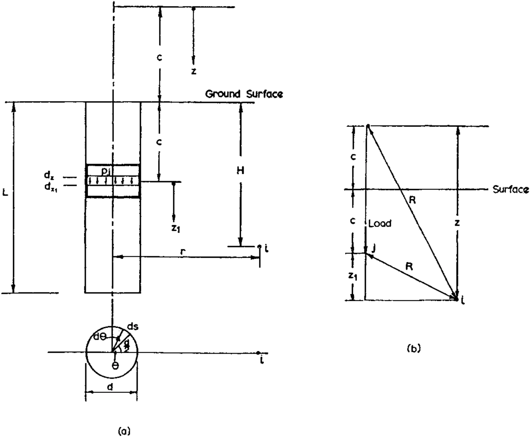
As described by Poulos and Davis (Ref. 10), the integration with respect to is done analytically, while the integration with respect to is done numerically.
Similarly, the influence factor for vertical displacement at due to the uniform base stress is given by
where is given by Eq. (2).
The integration is done analytically with respect to r and numerically with respect to .
The displacement at point due to all elements of the pile is then given by
Values of Pi and Pb have been obtained for various values of Lid by Poulos and Davis (Ref. 10) for incompressible piles, and Mattes and Poulos (Ref. 5) for compressible piles. In the latter paper, the relative compressibility of the pile is defined by the pile stiffness factor , where . The larger , the less compressible is the pile. These values have been used with the values of Iii and lib calculated from Eqs. (1) and (3) to obtain displacement distributions for a wide range of cases. In evaluating and , intervals of have been used for the numerical integrations. In all cases computed, has been taken equal to .
3.—DISPLACEMENT DISTRIBUTIONS DUE TO A SINGLE LOADED PILE
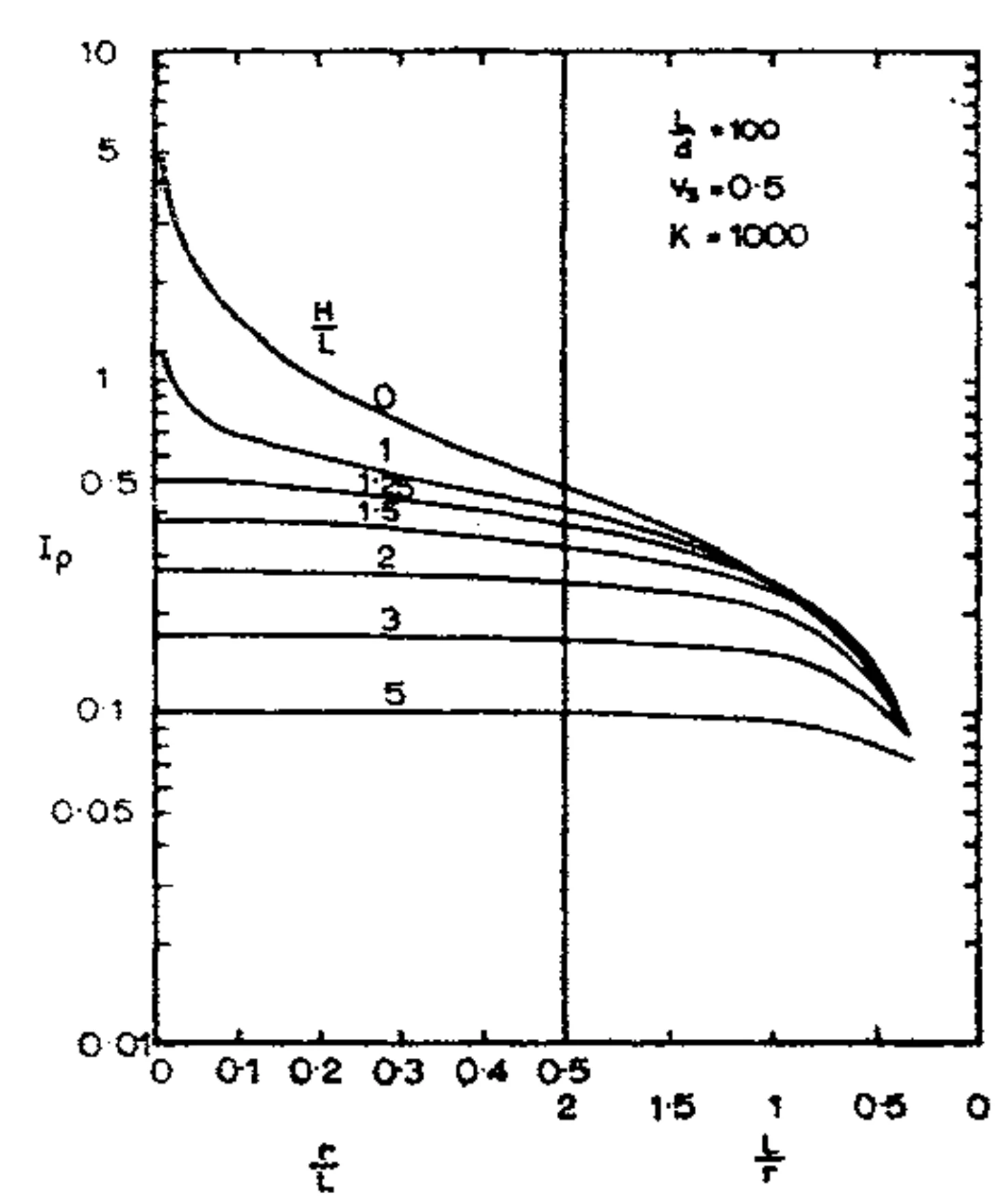
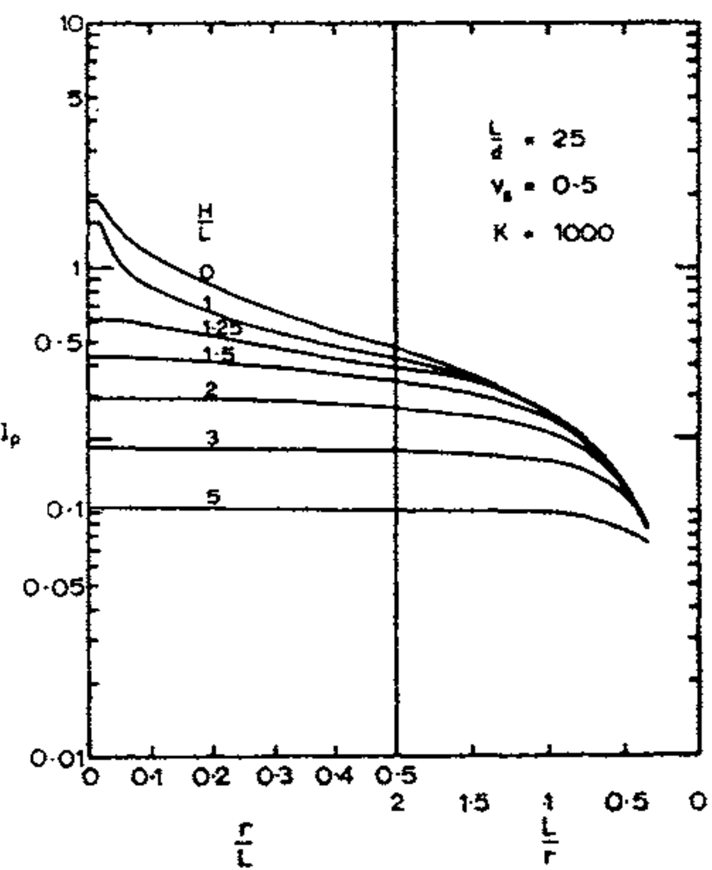
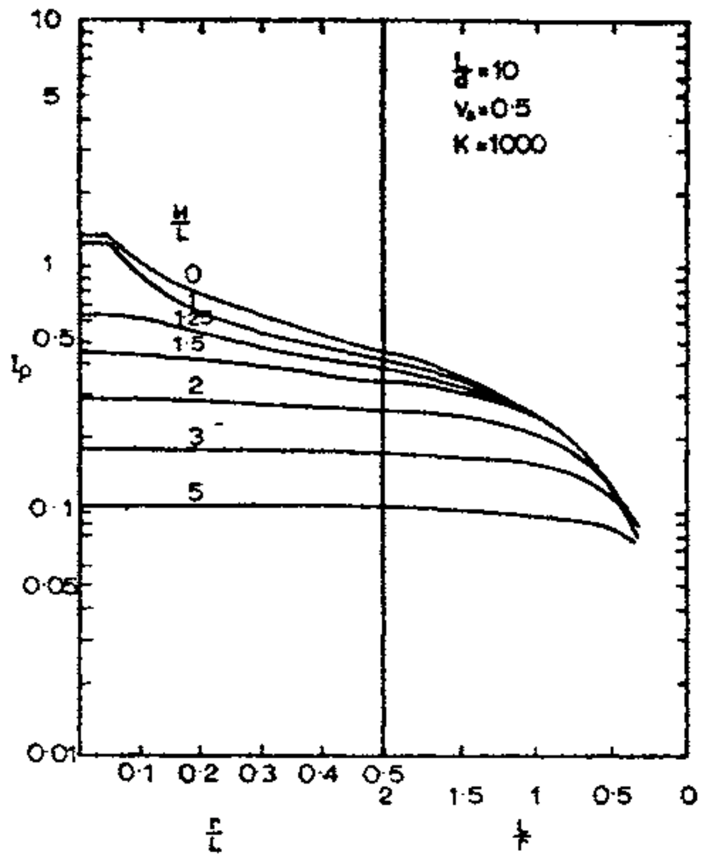
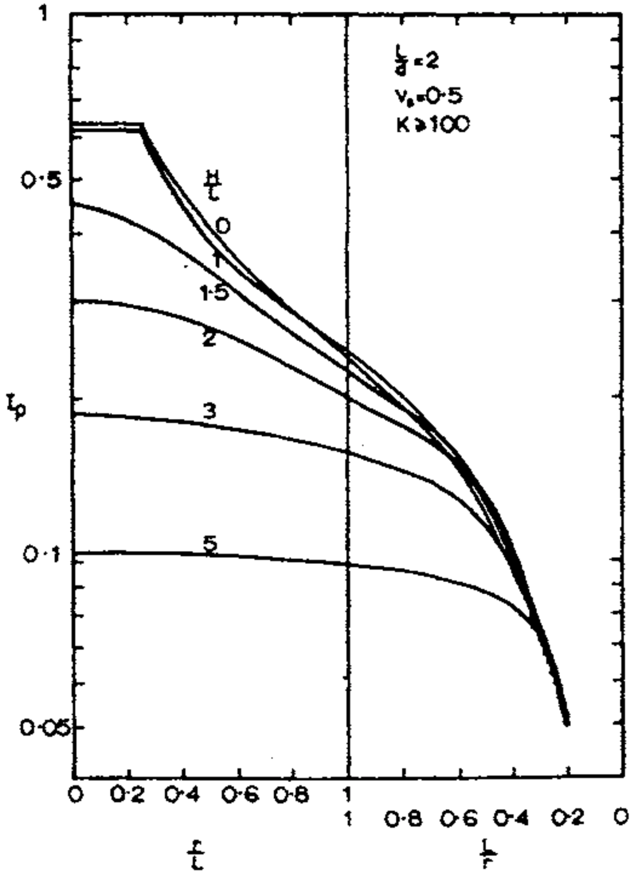
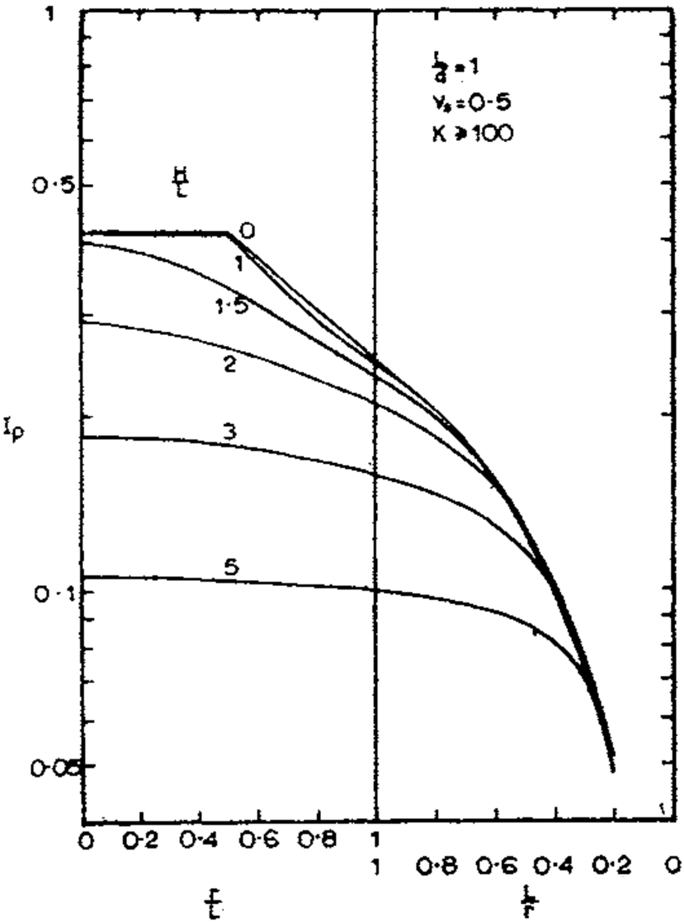
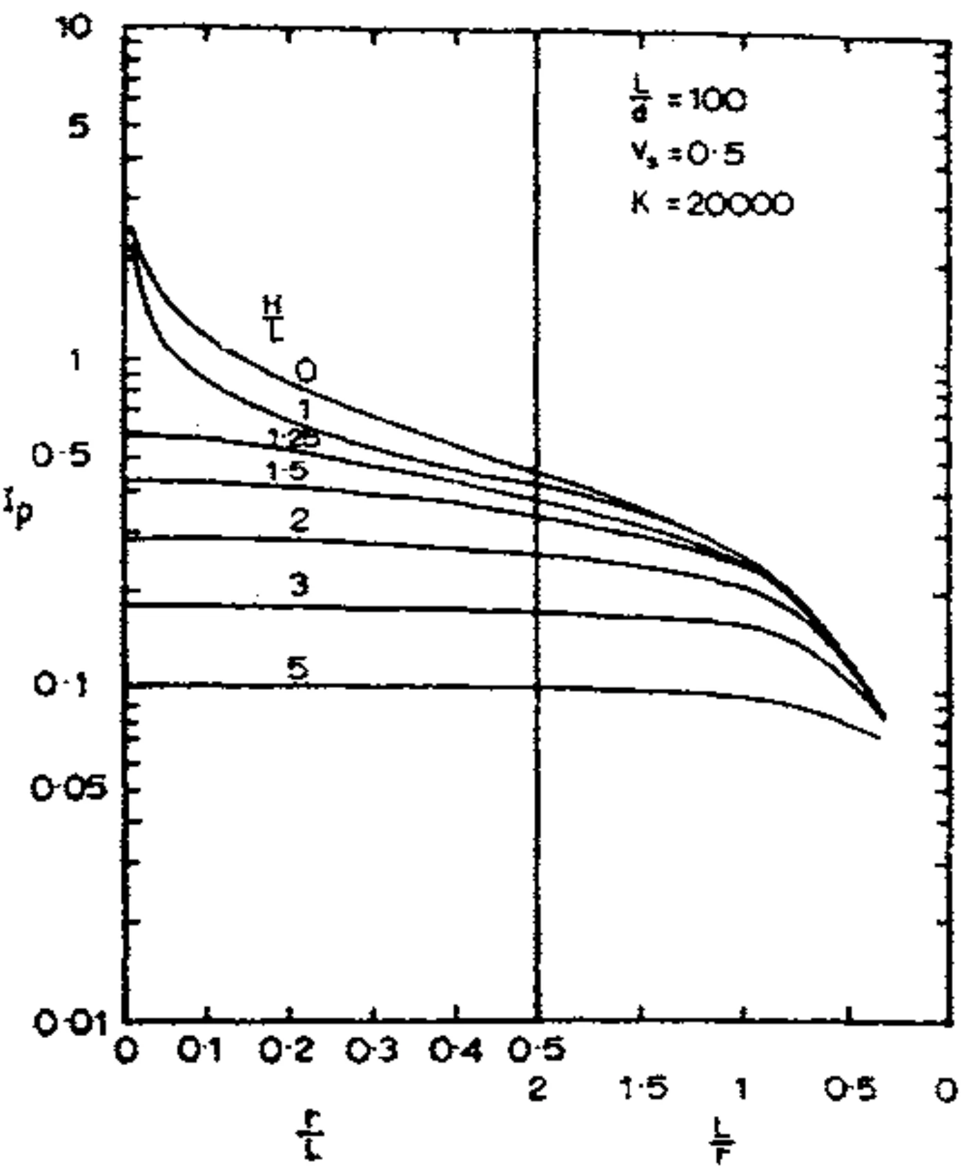
Influence factors for the displacement due to a single loaded pile have been obtained for values of ranging from 1 to 100 and are shown in Figs. 2 to 7 for various dimensionless depths and radii , and for . The actual displacement is given by
In Figs. 2 to 6, , while in Fig. 7, values of are given for , for . has a considerable influence on the displacements near the pile for , increasing as decreases, but only a small influence for or at points remote from the pile. The influence of on is relatively small, especially for , so that for practical purposes, the values of for may be used for all values of .
For points remote from the axis, it is foUnd that the pile may be replaced by a point load of magnitude equal to the load on the pile, and acting at a depth of 2/3L below the surface. The Mindlin equation for vertical displacement due to a point load may then be used, viz.,
where is the total load on the pile, and is defined in Eq. (2).
On the soil surface (), this equation reduces to the following simple form:
where .
It is found that for , the surface displacement calculated from Eq. (7) gives a value which agrees to within ± 3% of the more correct value calculated from Eq. (4), provided that . Even for shallow piers (e.g., ), the use of Eq. (7) for surface displacements gives results almost identical with the more correct analysis for .
4.—DETERMINATION OF SURFACE DISPLACEMENT PROFILE DUE TO A PILE GROUP
The displacement distributions for a single pile in Figs. 2 to 7 may be used to determine the surface displacement profiles due to a loaded pile group by superposition of the displacements due to each individual pile in the group at the point in question. Thus, for a group of n piles situated in a deep homogeneous soil layer, the displacement at a point on the soil surface is
where
is the load on pile ,
is the displacement influence factor , for , corresponding to the distance between the centre of pile and the point .
It should be noted that in this method, no account can be taken of the reinforcing effect of any piles which may be present between the point and the pile . The presence of such piles will tend to decrease the influence of pile on the displacement at and hence the displacement will be over-estimated by using Eq. (8). Some indication of the extent to which the displacement may be overestimated may be inferred from Fig. 8 (see later) which suggests that the overestimate will be relatively small.
If the pile group is situated on a finite layer of depth , which is underlain by a rigid base, the Steinbrenner approximation (Ref. 13) may be used to estimate the displacements. In this case,
where I is the value of for and for the value of equal to the distance between the centre of pile and the point .
The work of Davis and Taylor (Ref. 2) and Poulos (Ref. 8) in connection with surface footings suggests that the above approximation will be reasonably accurate in the vicinity of the pile but may be inaccurate remote from the pile (e.g., for ) or for very shallow layers.
If the pile group has a rigid cap, the distribution of loads Pi within the group will generally be non-uniform. This load distribution may be calculated by the method described by Poulos (Ref. 9) and Poulos and Mattes (Ref. 12). For square groups of incompressible piles, values of Pi are tabulated by Poulos (Ref. 9) for , and groups for , while some load distributions for groups of compressible floating piles are presented by Poulos and Mattes (Ref. 12).
In cases in which the load distribution within a group is not available or where a rough estimate only of the surface displacement is required, it is more convenient to assume a uniform distribution of pile loads (i.e., ) or else, if the group is large, to consider it as an equivalent single pier. In the latter case, the diameter of the pier should be taken such that the cross-sectional area of the equivalent pier equals the gross plan area of the group while the equivalent length of the pier may generally be taken in the range 0.6L to 0.9L (Ref. 9).
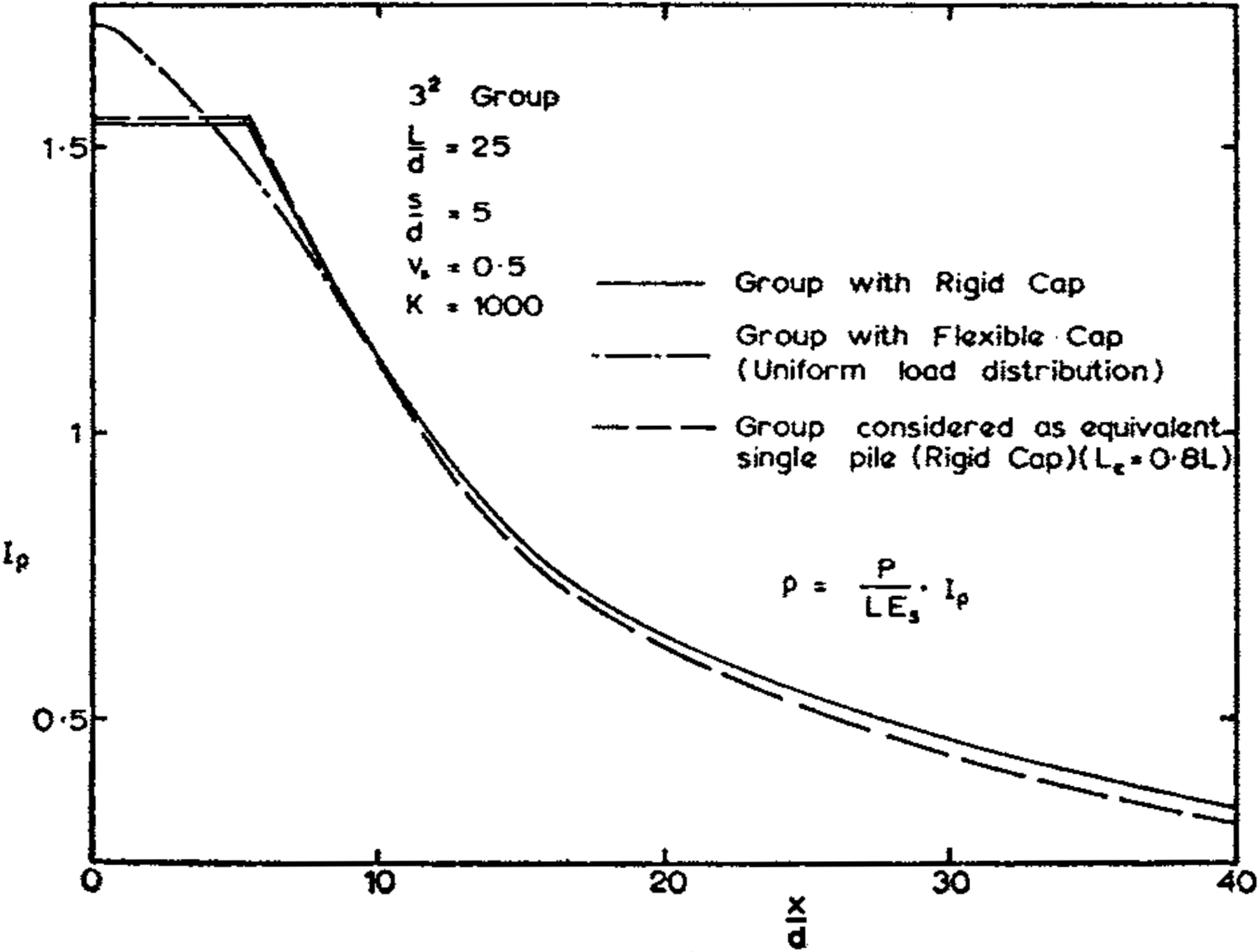
For a square group of 9 piles with a centre-to-centre spacing of 5 dia., Fig. 8 shows a typical comparison between the surface displacement profile for the group with a rigid cap, calculated from Eq. (9), that calculated by assuming the pile loads in the group are equal (i.e., that the pile cap is perfectly flexible) and that calculated by assuming the group to have a rigid cap and to be a single equivalent cylindrical pier of equivalent length . It will be seen that there is close correspondence between all three displacement profiles away from the immediate vicinity of the group. Underneath the pile group, the displacement distribution for the case of equal loads in all piles is not uniform and hence there is some difference between this case and the other two curves for a rigid pile cap. However, the differences are localised and for , the surface displacement profile for equal pile loads is virtually identical with that for the case of a rigid pile cap. Remote from the group, there is, however, a small discrepancy between the profile for the equivalent single pier and the profiles calculated for the actual group, the displacements in the latter case being greater than those for the equivalent pier. This discrepancy may possibly reflect the small order of overestimation of displacement involved in neglecting the reinforcing effect of intervening piles when using Eq. (9).
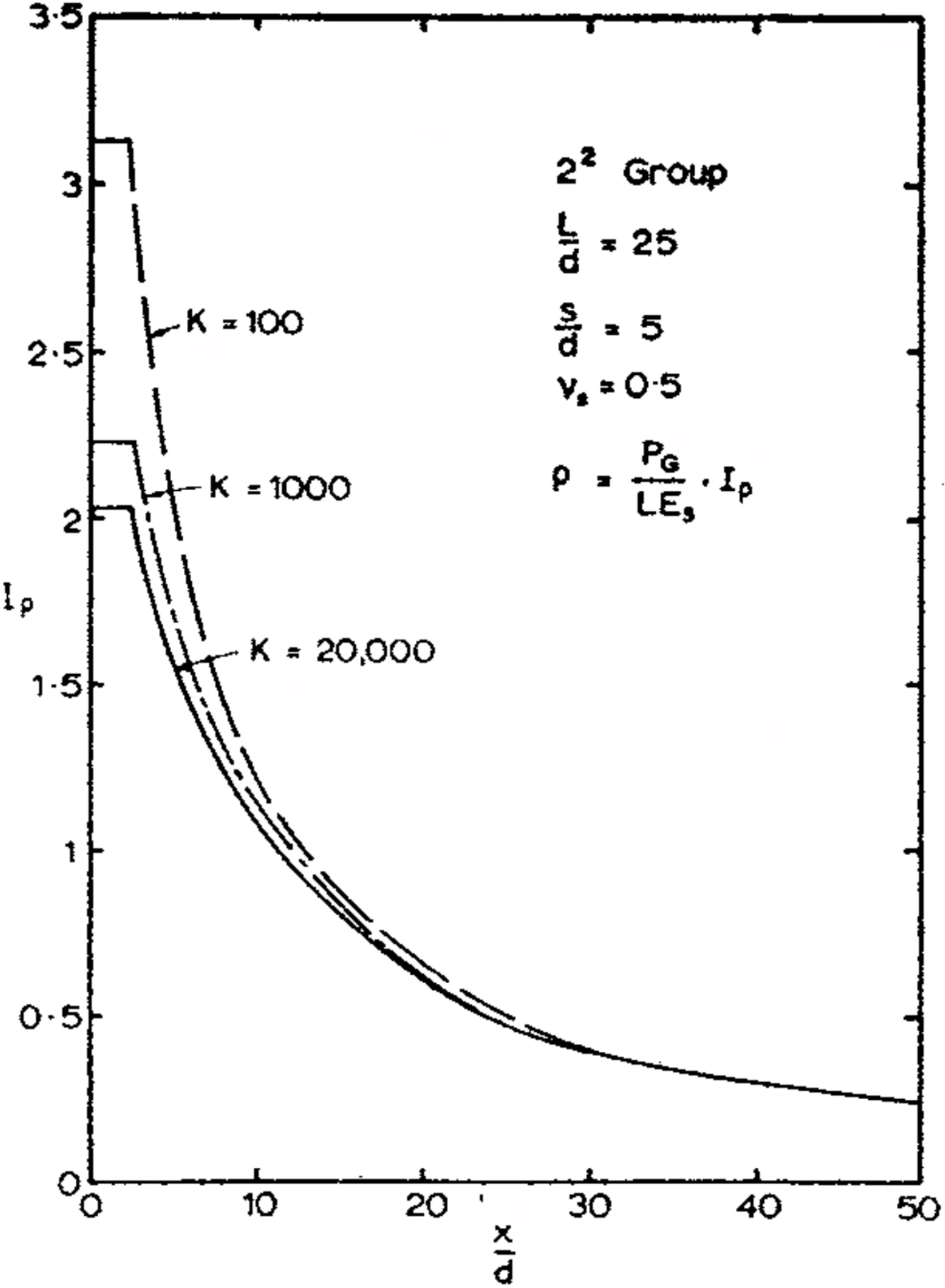
Typical surface displacement profiles are shown in Fig. 9 for a square four-pile group ( group) in a semi-infinite mass. The increased displacements with decreasing values of are clearly shown. However, for , the surface displacements are almost independent of .
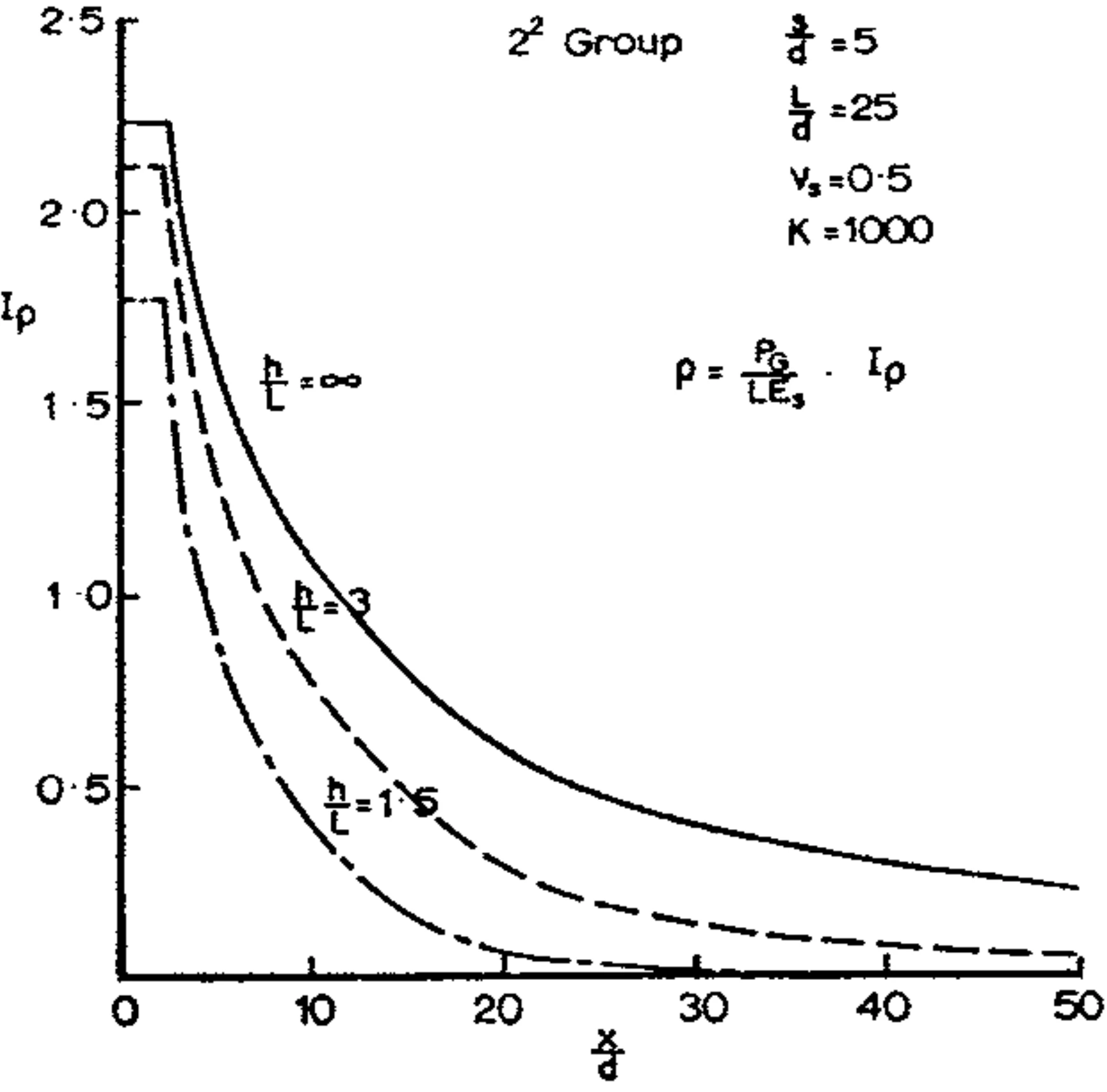
The influence of the layer depth on the surface displacement profile is shown in Fig. 10 for a group. As the layer depth decreases, the surface displacements are “damped” and, for relatively shallow layers (e.g., ), may be negligible at distances of one pile length or more from the centre of the group.
5.—DETERMINATION OF SETTLEMENT OF PILES AND PILE GROUPS UNDERLAIN BY LAYERED STRATA
The method outlined in the previous section for calculating surface displacement may be extended to the case where a pile or pile group is founded in a homogeneous layer which is underlain by further layers of different soils. In this case, the settlement may be calculated approximately by adding to the settlement of the pile or pile group in the founding layer, the contributions of the underlying layers.
Considering first the case of a single pile founded in a uniform layer of depth , a convenient method of calculating the settlement of the pile is as follows:
where
displacement influence factor for a pile in a layer of depth (obtained from Poulos and Davis (Ref. 10) for incompressible piles, Mattes and Poulos (Ref. 5) for compressible piles or Poulos and Mattes (Ref. 11) for end-bearing piles),
displacement influence factor on the pile axis at the level of the top of layer (obtained from Figs. 2 to 7),
Young’s modulus of layer ,
total number of different layers (including the founding layer).
The above method of calculation is similar to that suggested by Nair (Ref. 7) for piles and that used by Egorov et al (Ref. 3) for surface foundations and, in effect, makes use of the Steinbrenner approximation for the calculation of the displacements of the underlying layers.
Before proceeding, it is useful to consider briefly the limitations of Eq. (10) to calculate settlements. The major limitation is that no account is taken of the influence of changes in stress distribution below the pile which may occur because of the layering of the soil profile. In particular, if a stiffer layer overlies a softer layer, some concentration of stress into the stiffer layer will occur. Although the influence of such stress concentration on pile behaviour cannot readily be determined at the present time, some idea of the errors involved in using Eq. (10) may be obtained by considering the case of a circular surface footing on a two-layer elastic system underlain by a rough rigid base. It is found that the displacements calculated from Eq. (10) are generally greater than the more correct values, (obtained either from Burmister (Ref. 1) or from Odemark’s method, quoted by Ueshita and Meyerhof (Ref. 14». The errors are greatest when a stiff layer of considerable thickness overlies a thick softer layer, but unless the ratio of the Young’s moduli of the upper and lower layers IS greater than about 10, the resulting overestimate is. not serious. Furthermore, if softer layers overlie stiffer layers, Eq. (10) gives a displacement which agrees closely with the correct value.
A further limitation of Eq. (10) is that it inherently assumes that the shear stress distribution along the pile is that for a pile in a semi-infinite homogeneous soil mass and is unaffected by any heterogeneity of the soil below the pile. For cases involving different soil layers at some depth below the pile tip, the above assumption should be satisfactory as it has been found by Poulos and Davis (Ref. 10) that the shear stress distribution remains substantially unchanged if a rigid base exists below the tip of the pile. However, the approximation may be in error if the pile bears directly on to a stratum of considerably greater stiffness than the upper layer. The distribution of shear stress along the pile in this case may be considerably different from that for a pile in a semi-infinite mass, especially if the pile is relatively incompressible (Poulos and Mattes, Ref. 11). In such a case, the displacement factor for the pile in the upper layer of depth should be calculated from the solutions for an end-bearing pile presented by Poulos and Mattes (Ref. 11). The displacement factors for the underlying layers are calculated as before.
It therefore appears that Eq. (10) will give a reasonable estimate of the settlement of the pile unless a very stiff layer of considerable thickness beneath the pile overlies a very soft layer. The error involved in using Eq. (10) will generally lead to an overestimate of the settlement.
The calculation of the settlement of a single pile from Eq. (10) may be extended to the case of a pile group. For a group of n piles situated in a homogeneous layer of depth , underlain by a series of other strata, the displacement at the centre of the pile group can be calculated by summation of the settlement of the underlying layers due to all piles in the group. Thus
where
displacement of the pile group in a layer of depth and Young’s modulus which is underlain by a rigid base,
load in pile ,
displacement influence factor beneath the centre of the pile group for the level of the top of layer due to pile (obtained from Figs. 2 to 7).
The value of may be calculated as
where
the settlement ratio of group settlement to the settlement of a single pile under the same average load as a pile in the group,
settlement of single pile at the average pile load.
For a floating pile group, may either be calculated from the influence factors presented by Poulos and Davis (Ref. 10) or Mattes and Poulos (Ref. 5), or from a field load test on a single pile. may be calculated by the method described by Poulos (Ref. 9). For a group which rests on a firmer stratum below which a softer layer exists, may be calculated from the influence factors presented by Poulos and Mattes (Ref. 11), or again from a field load test, while may be calculated, as if the group was end-bearing, by the method described by Poulos and Mattes (Ref. 12).
For a pile group with a rigid cap, the values of in the group will not be uniform, as previously mentioned. The load distributions obtained by Poulos (Ref. 9) and Poulos and Mattes (Ref. 12) for a pile group in a homogeneous mass may be used to obtain values of although some slight inaccuracy may result because of the influence of the underlying compressible layers in modifying the load distribution. However, as shown in the previous section, little error will ensue if the load distribution within the group is assumed uniform. Alternatively, and again more expediently, the pile group may be replaced by an equivalent single pier as previously outlined. A further advantage of this latter method is that, for the relatively small value of which the equivalent pier will have, the values of will be almost independent of and thus it will generally not be necessary to consider different values of for different layers.
An example is given below of the calculation of the settlement of a floating pile group using both the correct . load distribution and a uniform load distribution in the group and also replacing the group by an equivalent single pier. An example is also given of the settlement calculation for a group which rests on a firmer stratum below which a softer layer exists.
6.—ILLUSTRATIVE EXAMPLES
6.1 Floating Pile Group:
The example considered is shown in Fig. 11. A group of concrete piles with a rigid cap is founded in a soil layer which is underlain by a further three layers and it is desired to calculate the settlement of the pile group. The values of Young’s modulus of the soil layers are given in Fig. 11 and are taken to be average values of the Young’s modulus of the soil skeleton so that the settlements calculated will be total final settlements.
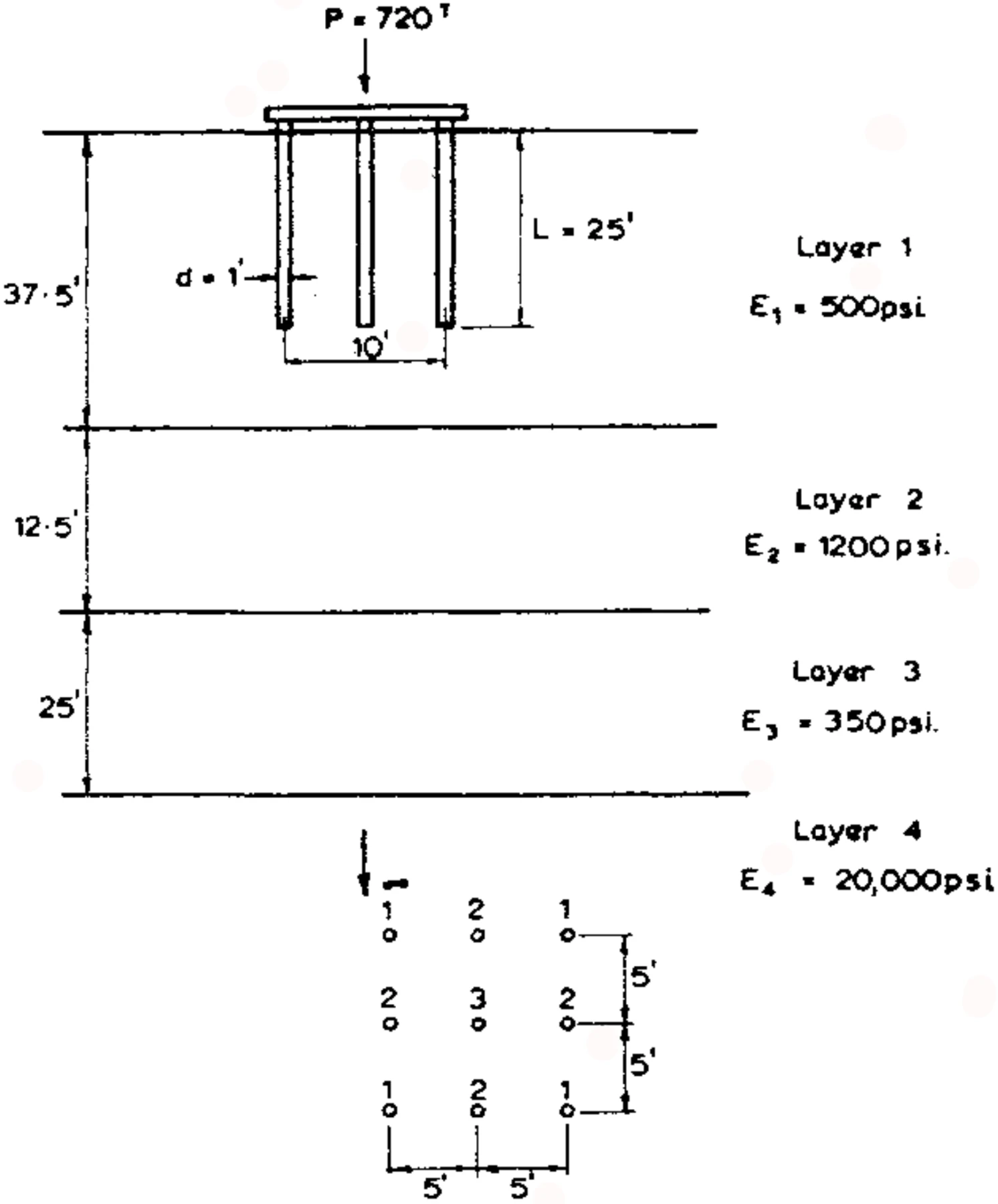
The settlement of the pile group in layer 1 may be calculated from Eq. (12). For the piles in layer 1, assuming of the concrete to be lb./sq. in., . For this value of , the piles may be considered incompressible (Mattes and Poulos, Ref. 5). From the influence factors given by Poulos and Davis (Ref. 10), for and , . For the pile spacing of , the value of is estimated from the results of Poulos (Ref. 9) to be 2.3. Hence the settlement of the pile group in layer , where is the total load on the pile group.
In order to calculate the additional settlements due to the underlying layers, three alternative methods will be used. Firstly, the correct non-uniform load’ distribution in the group will be considered; secondly, it will be assumed that the load distribution in the group is uniform; thirdly, the group will be replaced by an equivalent single pier.
(i) Considering Non-Uniform Pile Loads
From the tabulated results presented by Poulos (Ref. 9), the load distribution in the group may be obtained. The average pile load , and using the key to the piles shown in Fig. 11, the pile loads are as follows:
Since the settlement beneath the centre of the group is required, only three piles of the group need be considered because of symmetry. Because of the relatively large values of involved in this problem, the displacement influence factors are unaffected by the value of . The calculations are shown in Table I. The total additional settlement due to the underlying layers is found to be 2.25 in. The overall settlement of the group is therefore 3.78 + 2.25 = 6.03 in.
(ii) Considering Uniform Pile Load Distribution
In this case, the load on each pile is 80 tons. From Table I, the values of may be extracted for each pile and each layer. The resulting calculations are shown in Table II. In this case, the settlement of the group is 3.78 + 2.29 = 6.07 in. It will be seen that the calculated settlement is almost identical with that calculated from Table I using the correct non-uniform pile load distribution.
(iii) Considering the Group as an Equivalent Single Pier
The gross plan area of the group = 11 x 11 = 121 sq. ft. Therefore the equivalent diameter of a single pier de = 12.4 ft. From Poulos (Ref. 9), the equivalent length Le of the pier may be taken as 0.8L = 20 ft.
Eq. (10) may now be used to determine the settlement of the underlying layers. Since values of Ip are only given for L/d = 1 and L/d = 2, the values of I for the required value of Lelde = 1.6 will be interpolated from the value/for L/d = 1 and 2. The calculations are shown in Table III. Because the settlements are calculated beneath the centre of the group, only values of I p for r / L = 0 are required. The settlement of the group in this case is 3.78 + 2.52 = 6.30 in.
The calculated additional settlement due to the underlying layers from Table III is about 10% greater than the values calculated by the two previous methods. Nevertheless, the agreement is sufficiently good to suggest that, for a group containing a large number of piles, the replacement of the group by an equivalent single pier provides a convenient and reasonably accurate method of calculating the settlement of the group.
TABLE I
| Pile No. | Pile Load (tons) | Layer 2 | |||||
|---|---|---|---|---|---|---|---|
| 1 | 106 | 0.28 | 1.5 | 0.400 | 2 | 0.285 | 24.6 |
| 2 | 67 | 0.20 | 1.5 | 0.410 | 2 | 0.285 | 15.7 |
| 3 | 28 | 0 | 1.5 | 0.435 | 2 | 0.285 | 7.3 |
| Pile No. | Pile Load (tons) | Layer 3 | |||||
|---|---|---|---|---|---|---|---|
| 1 | 106 | 0.28 | 2 | 0.285 | 3 | 0.175 | 74.5 |
| 2 | 67 | 0.20 | 2 | 0.285 | 3 | 0.180 | 45.0 |
| 3 | 28 | 0 | 2 | 0.295 | 3 | 0.185 | 19.7 |
| Pile No. | Pile Load (tons) | Layer 4 | ||
|---|---|---|---|---|
| 1 | 106 | 3 | 0.175 | 2.1 |
| 2 | 67 | 3 | 0.180 | 1.4 |
| 3 | 28 | 3 | 0.185 | 0.6 |
For layer 2, Settlement
For layer 3, Settlement
For layer 4, Settlement
Total settlement of layers 2 to 4
TABLE II
| Pile No. | Values of | ||
|---|---|---|---|
| Layer 2 | Layer 3 | Layer 4 | |
| 1 | 18.8 | 56.2 | 1.6 |
| 2 | 18.8 | 54.7 | 1.7 |
| 3 | 20.8 | 56.3 | 1.7 |
For layer 3, settlement
For layer 4, settlement
Total settlement of layers 2 to 4
TABLE III
| Layer 2 | |||||
|---|---|---|---|---|---|
| 1 | 1.88 | 0.186 | 2.5 | 0.136 | |
| 2 | 1.88 | 0.486 | 2.5 | 0.300 | |
| 1.6 (by linear interpolation) | 1.88 | 0.355 | 2.5 | 0.235 | 0.223 |
| Layer 3 | |||||
|---|---|---|---|---|---|
| 1 | 2.5 | 0.136 | 3.75 | 0.082 | |
| 2 | 2.5 | 0.300 | 3.75 | 0.180 | |
| 1.6 (by linear interpolation) | 2.5 | 0.235 | 3.75 | 0.141 | 0.601 |
| Layer 4 | |||
|---|---|---|---|
| 1 | 3.75 | 0.082 | |
| 2 | 3.75 | 0.180 | |
| 1.6 (by linear interpolation) | 3.75 | 0.141 | 0.16 |
For layer 3, settlement
For layer 4, settlement
Total settlement of layers 2 to 4
The above example emphasizes that compressible layers well beneath the pile group may contribute significantly to the settlement of the group. In this case, the additional settlement due to the underlying layers comprises about 37% of the overall settlement. The example also highlights the possible consequence of incomplete site investigation.
6.2 End-Bearing Pile Group:
The problem is shown in Fig. 12. A group of concrete piles is founded through alluvial clay on to a medium dense sand, which is underlain by a soft clay layer which rests on shale. Average values of both undrained Young’s modulus and Young’s modulus of the soil skeleton are given and both the immediate and total final settlements are calculated. Because the displacement influence factors are not seriously influenced by Poisson’s ratio (see Section 3), it has been assumed that, under both undrained and drained conditions, values are those for .
The group is considered first as end-bearing. The value of of the piles is about 6,000, so that from the results of Poulos and Mattes (Ref. 11), such piles are virtually incompressible, and hence the settlement of a single pile is merely the elastic settlement of the pile itself. Furthermore, from the results of Poulos and Mattes (Ref. 12), no interaction occurs between adjacent piles, i.e., , and all piles are equally loaded**.
**Because the supporting sand layer is not perfectly rigid, some interaction may in fact occur, but it is unlikely to be significant.
Hence, the settlement of the piles, when considered as bearing on a rigid stratum, is
where
is the average pile load,
is the area of the pile,
is Young’s modulus of the pile.
In this case, it is found that, for
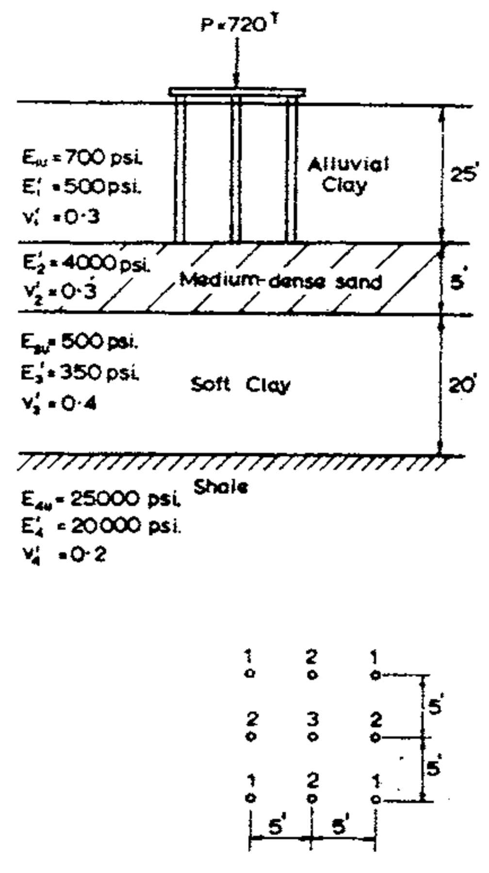
The calculation of the additional settlements due to the underlying layers is shown in Table IV. The settlement of the sand layer is assumed to occur immediately. The immediate settlement of the group is the sum of the elastic pile settlement and the immediate settlement of the underlying layers, i.e., 0.16 + 3.21 = 3.37 in. The total final settlement is 0.16 + 4.46 = 4.62 in. Thus, because of the underlying soft. clay layer, a considerable amount of consolidation settlement (1.25 in.) occurs in this case, whereas if the pile were founded on a truly rigid stratum, only an immediate settlement of 0.16 in. would occur.
7.—COMPARISON WITH FIELD CASE
As an indication of the applicability of the method described to field situations, an attempt was made to compare the measured settlements of the furnace foundation described by Golder and Osler (Ref. 4) with the calculated values. The foundation supported a total load of 2,400 tons and consisted of 32 Franki piles of 22-ft. length arranged in a generally rectangular pattern consisting of 3 interior rows of 8 piles each, the rows spaced at 10.5 ft. and the piles at 6 ft., and at each end, 4 piles spaced at 7-ft. centres. The soil profile could generally be characterised as about 95 ft. of sand interspersed with layers of silty clay and sandy clay, and underlain by a very deep deposit of a firm grey silty clay (Leda clay).
A single pile test was carried out and revealed that, under the average working load, the single pile settlement was about 0.04 in. An analysis carried out, as described by Poulos (Ref. 9), gave a value of settlement ratio of the pile group in the sand of 8.5. Thus, the settlement of the piles in the sand () is 8.5 x 0.04 = 0.34 in.
Considering now the settlement due to the Leda clay, only oedometer results are given for this clay and it is therefore necessary to use these results to estimate Young’s modulus of the clay. The data given is compression index , and void ratio = 1.25. From these results, a value of the coefficient of volume decrease may be derived for a typical depth of say 50 ft. below the sand-clay interface. This gives Using now the theory for an ideal elastic soil,
Assuming a typical value of for the firm clay of 0.2, it is found that Considering now the calculation of the settlement due to the clay, and assuming the clay to be semi-infinite, it is found that the settlement is 3.3 in. Thus, the total settlement of the group is 3.3 + 0.34 = 3.7 in.
The actual foundation was in fact demolished before the final settlement had been attained, at which time, the measured settlement had reached about 1.8 in. Measured values of the coefficient of consolidation cv vary too widely to be able to accurately estimate the degree of settlement at the time of demolition. However, if an average value of cv of . is assumed, the dimensionless time factor (assuming the foundation to be replaced by an equivalent circular foundation of radius ) after 11 years is 0.91. From the three-dimensional rate of settlement analysis of Mandel (Ref. 6) for a circular foundation on a sand layer overlying a deep clay layer, it is found that the appropriate degree of settlement is about 0.38. Thus, the estimated final settlement (taking account of an initial sand settlement of 0.5 in.) = (1.3/0.38) + 0.5 = 3.9 in., which is in general agreement with the calculated value. In addition, the initial settlement of the group, of about 0.5 in., due largely to the sand, is consistent with the calculated value of of 0.34 in.
Although the settlements calculated by the method in this paper are very similar to those produced by Golder and Osler using one-dimensional theory, the present method would appear somewhat more logical as it does not require any arbitrary selection of rigid boundaries beneath the clay or reductions for foundation rigidity as is the case with the one-dimensional predictions.
8.—CONCLUSIONS
Distributions of vertical displacement within a semi-infinite mass due to a loaded pile have been obtained for various length-to-diameter ratios of the pile. It has been found that, even at points relatively close to the pile, the displacements due to a pile agree closely with those due to an equivalent single point load acting at a depth of two-thirds of the pile length. A method of calculating the surface displacement profile around a pile group and the settlement of a pile group underlain by layered strata, using the single pile displacement distributions, has been suggested. It has been found that, for a pile group having a rigid pile cap, the displacements may be calculated with sufficient accuracy by assuming all piles are equally-loaded and ignoring the correct non-uniform load distribution within the group. The replacement of the pile group by an equivalent single pier has been shown to lead to an estimate of the displacement which is quite adequate for practical purposes. Such a procedure appears to be most convenient when considering displacements due to a group containing 3 large number of piles.
ACKNOWLEDGMENTS
The work described in this paper forms part of a general programme of research into the settlement of all types of foundations, under the general direction of Professor E. H. Davis, whose comments are gratefully acknowledged. The work was carried out in the School of Civil Engineering at The University of Sydney, the Head of which is Professor J. W. Roderick, and was supported by a grant from the Australian Research Grants Committee. The computational work was carried out using the facilities of the Basser Computing Department of the School of Physics at the University of Sydney.
References
- BURMISTER, D. M.-The Theory of Stresses and Displacements in Layered Systems and Applications to the Design of Airport Runways. Proc. Highway Research Board, Vol. 23, 1943, pp. 126-48.
- DAVIS, E. H. and TAYLOR, H.-The Movement of Bridge Approaches and Abutments on Soft Foundation Soils. Proc. First Conf. Aust. Road Research Board, Canberra, 1962, Vol. I, Part 2, pp. 740-64.
- EGOROV, K. E., KUZMIN, P. G. and POPov, B. P.-The Observed Settlements of Buildings ‘as Compared with Preliminary Calculation. Proc. Fourth Int. Conf. Soil Mechanics and Foundation Engg., London, 12-24 August, 1957. London, Butterworth, 1957, Vol. I, pp. 291-6. 35
- GOLDER, H. Q. and OSLER, J. C.-Settlement of a Furnace Foundation, Sorel, Quebec. Canadian Geotech. Jour., Vol. 5, No. I, Feb., 1968, pp.46-56.
- MATTES, N. S. and POULOS, H. G.-The Settlement of a Single Compressible Pile. Proc. A.S.C.E., Jour, Soil Mechanics and Foundations, Div., Vol. 95, No. SM1, Jan., 1969, pp. 189-207.
- MANDEL, J.-Tassements produits par la consolidation d’une couche d’argile de grande epaisseur. Proc. Fifth Int. Conf. Soil Mechanics and Foundation Engg., Paris, 17-22 July, 1961, Vol. 1, pp. 733-6.
- NAIR, K.-Load Settlement and Load Transfer Characteristics of a Friction Pile Subject to a Vertical Load. Proc. Third Pan-American Conf. Soil Mechanics, Caracas, Venezuela, 1967, p. 565.
- POULOS, H. G.-Stresses and Displacements in an Elastic Layer Underlain by a Rough Rigid Base. Geotechnique, Vol. 17, No.4, 1967, pp. 378-410.
- POULOS, H. G.-Analysis of the Settlement of Pile Groups. Geotechnique, Vol. 18, No.4, 1968, pp. 449-71.
- POULOS, H. G. and DAVIS, E. H.-The Settlement Behaviour of Single Axially-Loaded Incompressible Piles and Piers. Geotechnique, Vol. 18, No.3, 1968, pp. 351-71.
- POULOS, H. G. and MATTES, N. S.-The Behaviour of Axially Loaded End-Bearing Piles. Geotechnique, Vol. 19, No.2, 1969, pp. 285-300.
- POULOS, H. G. and MATTES, N. S.-Settlement and Load Distribution Analysis of Pile Groups. Aust. Geomechanics Jour., Vol. G1. No.1, 1971, pp. 18-28.
- STEINBRENNER, W.-Tafeln zur Setzungberechnung. Die Strasse, Vol. 1, 1934, p. 12l.
- UESHITA, K. and MEYERHOF, G. G.-Deflection of Multilayer Soil Systems. Proc. A.S.C.E., Jour. Soil Mechanics and Foundations Div., Vol. 93, No. SM5, Sept., 1967, pp. 257-82.