Complex Flow through Porous Media
1. Introduction
1.1 General:
By definition, a porous medium is an assembly of solid particles or grains which encloses a system of interconnected voids through which a fluid may flow under the influence of an appropriate pressure gradient.
Such media are therefore particulate in nature and any attempt to describe their internal geometry in detail is fraught with virtually insurmountable complexity.
As a statement of boundary geometry is essential to all solutions involving theoretical mechanics, the prospect of representing exactly the flow of a fluid through such a medium is remote.
In common with other problems involving the transport of physical phenomena such as heat, force, etc., through real materials a remarkable degree of success has been achieved during the past century or so by completely neglecting the complexity of internal geometry and adopting the concept of the equivalent continuum.
It is presumed that a representative sample of this continuum can be obtained and subjected to testing to ascertain average values of these properties which govern the particular behaviour under consideration.
In the case of flow through porous media Darcy (Ref. 1) is credited with being the first person to adopt this approach in his well known experiments involving seepage flow through a variety of sand samples which led to the identity now generally known as Darcy’s law-
in which = the superficial or average seepage velocity,
= the coefficient of permeability in the direction of flow,
= the (negative) total piezometric head gradient.
Slichter (Ref. 2) indicated that Eq. (1) did not hold for relatively high values of V. Slichter was particularly interested in the influence of pore geometry on the onset of turbulence and it became generally accepted that Darcy’s law is only applicable when the flow is laminar and breaks down on the onset of turbulent conditions.
Since that time a number of attempts have been made to develop improved relationships to describe flow through porous materials. They fall generally into two categories. First those which are an extension of Slichter’s approach in that they seek to use idealised physical models to describe the fluid behaviour in the pore space and second those which are of the continuum type but employ mathematical expressions more sophisticated than Darcy’s law to describe the flow through an “element”.
The first group may be further subdivided into the capillary theories and the hydraulic radius theories. Both find their origin in classical pipe and channel flow mechanics. The capillary theories assume that the pore space of a porous medium may be represented by a series of straight capillary tubes and the flow is assumed to be governed by the Hagen-Poiseuille equation. Examples of the use of this approach are given by Adzumi (Ref. 3), Childs and Collis-George (Ref. 4), and Marshall (Ref. 5).
The principal objection to the extrapolation of these methods outside the strict Darcy regime lies in the fact that inertial effects due to curvature of the fluid paths in real media are completely ignored. The hydraulic radius theories represent an advance in that inertial effects may be recognised although, until recently, they have not been taken into account.
Kozeny (Ref. 6) originally developed a hydraulic radius theory by considering the medium as an assemblage of channels of fixed length but of varying section. Carman (Ref. 7), Wyllie and Gregory (Ref. 8) also employ this approach and in 1956 Hubbert (Ref. 9) showed that, using a method analogous to Kozeny’s, Darcy’s law is valid only for flow velocities such that the inertial forces are negligible compared with those due to viscosity.
It may be noted that both Kozeny and Hubbert used the Navier-Stokes equations ignoring inertia terms to express the overall flow in the assumed channels.
Among the continuum flow equations two stand out.
In 1901, Forchheimer (Ref. 10) suggested a simple polynomial expression to describe the flow conditions-
where and are constants determined by the properties of the fluid and medium. Although Forchheimer subsequently added a third term in an attempt to obtain improved fit with experimental results, Eq. (2) is generally referred to as Forchheimer’s equation.
A number of workers have inferred that Forchheimer’s equation has sound physical backing apart from its attraction as a relatively simple non-linear expression.
Aravin and Numerov (Ref. 11) stated that from their investigations the soundest law both from theoretical and experimental viewpoints seemed to be the drag law of seepage which they gave as Eq. (2).
Ward (Ref. 12) derived an equation of the Forchheimer type from dimensional analysis and the results of experiments carried out by Lindquist (Ref. 13) can be expressed in this form.
One of the most important recent developments is due to Irmay (Ref. 14) who derived the Forchheimer relation by inferred argument from the fundamental Navier-Stokes equations for the general case when inertia terms are considered.
The second important flow relationship in this category is attributed to Missbach (Ref. 15) who suggested the use of an equation of the general form
where = constant determined by the properties of the medium and the fluid,
= an exponent with values lying between 1 and 2.
Eq. (3) has been used extensively by White (Ref. 16), Escande (Ref. 17), Wilkins (Ref. 18), Parkin et al (Ref. 19), and Anandakrishnan and Varadarajulu (Ref. 20).
Dudgeon (Ref. 21) carried out tests on coarse materials including a number of gravels, sands and packings of uniform spheres and confirmed that while the results followed closely expressions of the form of Eq. (3) the values of c and m were not constant for the one material for all flow conditions.
1.2 Watson’s Model:
A significant advance in the use of particulate models was introduced by Watson (Ref. 22). Extending an approach described by Philip (Ref. 23) he suggested the use of the regular “square” model shown in Fig. 1. Such an arrangement is essentially a clastic model as defined by Trollope (Ref. 24) and, following extensive analyses of its properties, which are to be described in this paper, it has been found to be of very great value in aiding the understanding of complex flow in porous media.
One of the most encouraging results of recent work is the demonstration that analysis of Watson’s model using the Navier-Stokes equations, including the inertia terms, leads directly to Forchheimer’s equation, thus linking the particulate and continuum approaches. It has also been shown that the terms and are subject to small variations depending on the Reynolds number of the flow regime which is in accord with Dudgeon’s experimental observations. In general however, when included in the Forchheimer expressions these variations are not likely to be of major practical significance.
2. The fundamental characteristics of flow through porous media
2.1 Flow Regimes:
It is convenient to classify flow regimes in terms of the behaviour of the fluid in the pore space, these are
- The pre-laminar regime,
- The laminar regime,
- The turbulent regime.
The pre-laminar regime is associated with very low velocities so that in these circumstances even water ceases to act as a Newtonian fluid. Such flows are frequently associated with extremely small pore sizes, e.g., in clay soils, and the physico-chemical interaction of particles and fluid then has a profound influence on the overall regime. Flows of this type are outside the scope of this paper.
The laminar regime is one where, under steady flow conditions an element of the fluid follows a smooth path. At first it was thought that Darcy’s law was valid for all laminar conditions. It is now understood however
It is useful to convert these equations into dimensionless form by that the laminar regime is always non-linear in character and that the use of the linear Darcy equation is a justifiable approximation only when the effect of the inertia terms in the Navier-Stokes equations is negligible compared with that of the viscosity terms. These conditions occur when the flow velocity is small and this is sometimes called “creeping flow”.
For practical purposes the linear approximation is useful for Reynolds numbers up to the order of unity and fortunately this covers a wide range of natural situations involving materials of particle size less than 1 mm.
It is clear however that the non-linear behaviour of laminar flows through porous media is a topic of considerable practical interest and importance and this paper is primarily concerned with theoretical and experimental evaluation of this phenomenon.
Not the least of the items of theoretical and practical significance is the fact that non-linear flow observations in these circumstances cannot necessarily be attributed to the onset of turbulence.
A turbulent regime develops at high Reynolds numbers when the fluid velocities are sufficient to cause instantaneous fluctuations or eddies in the flow path. Under these circumstances changes in flow characteristics with time must be considered and the solution of the fundamental Navier-Stokes equations is extremely difficult even for the simplest geometrical configurations.
Nevertheless the available evidence suggests that the continuum Eqs. (2) and (3) are sufficiently flexible to permit their use in turbulent conditions within porous media.
2.2 Theoretical Investigations of the Laminar Regime:
Fluid flow within the interstices of any porous material will be governed by the basic fluid mechanics relations-the Navier-Stokes equations. As the boundary conditions imposed by the irregularity of the pore spaces are, in general, highly complex and variable the governing equations, which in themselves are fourth order and nonlinear defy analytical solution. As previously noted however it is possible to
- consider numerical solutions within a porous medium with simplified or idealised boundary conditions (the particulate approach),
- derive the generalised flow equation in terms of the characteristics of the flow (such as those obtained from a solution of the Navier-Stokes equations) and the properties of the fluid and porous medium (the continuum approach).
Both approaches as developed in this paper start with the assumption that for compressible viscous flow the Navier-Stokes equations may be written as
and continuity gives
where the velocity , represents time, piezometric head is and the fluid has density , specific weight , dynamic viscosity , and kinematic viscosity .
If the velocity values are known throughout the flow field the pressure and piezometric head may be deduced at every point from these values and, further, the head gradient between any two points can then be evaluated.
For simplicity the relations will be deduced here for two-dimensional flows-the corresponding three-dimensional arguments are given as the Appendix.
For two-dimensional flow the velocity is given by
a stream function may be defined by
and the vorticity is given by
Using Eq. (8) the piezometric head gradients in the x- and y-directions are obtained from Eq. (4) as
and
It is useful to convert these equations into dimensionless form by introducing representative parameters (velocity) and (distance) such that
where the bar indicates a dimensionless quantity.
Reynolds number (RN) may then be defined in conventional fashion by
and the differential equations for the piezometric head gradient may be written in dimensionless form. Thus Eq. (9b) becomes
and a similar equation is obtained for the gradient in any pertinent direction.
It should be noted that the piezometric head gradient depends upon
- field variations of velocity (including vorticity),
- , and which are related, and
- and which are properties of the fluid.
Therefore to assist with the further analysis of this relation it is useful to write it in the form
where and are expressions (not usually constants) derivable from the characteristics of the flow patterns under study and dependent only on Reynolds numbers and the pore geometry.
The particulate approach is now followed by assuming a simplified void geometrY and solving Eq. (13) for these boundary conditions. If steady flow is considered, numerical solutions of the vorticity-transport equations (Ref. 25) will give the flow characteristics required to evaluate and throughout the flow. Such solutions were obtained by Stark (Ref. 26) for a variety of idealised particle arrangements and Figs. 2, 3, 4 and 5 show some typical stream-function solutions.
The continuum approach is one whereby the average properties within a pore space are assumed to pertain over the adjacent space and each pore is considered as an infinitely small element within the whole porous medium. Consider a typical pore space as shown in Fig. 6 in which the relevant properties of the continuum element shown dotted are given as and where is the seepage velocity and is the piezometric head drop gradient across the element.
Now if the representative velocity () used in the flow derivations is chosen as the seepage velocity it follows from Eq. (13) that if the distance is given by
where again and may be calculated for an idealised medium from the numerical solutions of the Navier-Stokes equation.
If a particular porous medium is considered (i.e., is fixed), and the fluid properties ( and ) are known then this relation reduces to
where and
It is important to note here that whereas and are functions of and the pore geometry only, is also a function of the pore (or particle) size while is a function of , pore geometry, pore (or particle) size and the fluid.
It is still necessary to consider a further two points,
- whether is in fact the appropriate representative head gradient across the pore space to be used in the continuum flow relations, and
- under what circumstances and may be assumed constants for a given fluid in a given porous medium.
- If the element illustrated in Fig. 6 is representative of the surrounding flow (and this is usually the case where the same macroscopic flow relations are used over extensive regions of the flow) then although, by virtue of the nonlinearity of the Navier-Stokes equations, , and will not be lines of symmetry (except when ) the flow patterns crossing and will show periodic similarity and, as the piezometric head gradients at a point are dependent only upon the surrounding velocity characteristics, it follows that the pressure drops between and are identical and therefore that the head gradients along , and any other line parallel to these and crossing the pore space will all be identical. Further, if the medium is isotropic and homogeneous, the same values for and will apply for any direction of flow.
- An examination of the streamline profiles obtained in the numerical solutions shows that over quite extensive ranges of there is little change in the dimensionless velocity characteristics—particularly in the main body of flow. Although the position of the separation streamline (separating the main flow from the wake flow) and the vortex patterns alter significantly with changes in they do not appear to have an important effect on the head gradient versus velocity relation unless the change in involves at least one order of magnitude. This observation is supported by a study of the numerically calculated gradients (Refs. 26 and 27) and is illustrated by considering the results (Table I) in which values of () (Eq. (14)) are tabulated for flow through the idealised model of Fig. 1 at three different pore geometries.
| 0.0 | 18.78 | 0.0 | 876.2 | 0.0 | 1.16 |
| 0.05 | 18.79 | 8.0 | 879.6 | 2.5 | 1.20 |
| 0.5 | 18.81 | 40.0 | 898.3 | 12.5 | 1.32 |
| 2.5 | 18.86 | 50.0 | 901.8 | 25.0 | 1.42 |
| 5.0 | 19.02 | 80.0 | 911.9 | 50.0 | 1.50 |
| 10.0 | 19.42 | ||||
| 15.0 | 19.80 | ||||
| 25.0 | 20.22 | ||||
| 50.0 | 20.82 | ||||
| 100.0 | 21.44 | ||||
| 150.0 | 21.62 | ||||
| 200.0 | 21.66 | ||||
Darcy Flow: In the limiting case when the particulate flow relation (13) and the continuum relation (15) reduce to their respective forms of Darcy’s equation which may be written in the form
in Darcy flow is assumed as a constant but the analyses above show that this is only an approximation. For creeping flows, however, where RN is approximately zero this assumption is well within experimental accuracy and has formed the basis of many studies of seepage flow.
The numerical studies suggest that the limit of validity of Darcy’s law depends upon the properties of the medium involved, however, generally it may be assumed to hold within ± 1 % if (based on seepage velocity and mean particle size) is less than 1. The solutions in Table I support this assumption.
If the continuum is considered then within this continuum the differential form of Darcy’s Law may be written
and this relation satisfies the potential definition for irrotational flow within the boundary conditions, and therefore satisfies Laplace equation
Thus all the solutions and methods of solution available for Laplace’s equation become available for finding the value of (and therefore ) at any point in the continuum.
It should be noted that the corresponding particulate equations do not satisfy potential flow requirements because the boundary conditions within the pore spaces must then satisfy “no slip” conditions.
Alternatively (in terms of stream-function) for creeping flow in the continuum and the boundary conditions of irrotational flow apply whereas for creeping flow within the pore spaces and “no slip” conditions apply on the particle boundaries.
2.3 The Forchheimer Relation:
The more general relation for laminar flow given by Eq. (15) is sometimes referred to as the non-linear laminar relation and the regime of flow for which this equation applies is the non-linear laminar or non-Darcy laminar regime. When and are considered as constants this equation becomes the Forchheimer relation. It should be noted then that just as Darcy’s equation applies over a limited range of with reasonable accuracy so too as explained above the Forchheimer relation will hold over limited ranges of within the laminar flow range. The actual flow range and accuracy with which a given set of values of and will apply will depend on the geometry of the pore space involved. As a guide, Darcy’s Law will generally hold for with an accuracy of ± 1 % whereas a Forchheimer relation can approximate with about the same accuracy for . Naturally, if the accuracy stipulated is reduced the applicable range of can be increased.
It follows therefore that whenever permeameter tests are performed on a given porous medium and a smooth curve is fitted to the results to obtain an appropriate value of and these values will have an accuracy dependent on the range of flows used in the tests. Further, such values should only be used in calculations involving Reynolds numbers appropriate to this range of flows. It is always inadvisable to extrapolate coefficients from a given series of permeameter tests.
2.4 Other Relations
Eq. (14) can be rewritten in the form
by assuming has a constant value where is the value obtained for when . If the permeability at any is defined by
then
This relation which Tek (Ref. 28) deduced empirically is essentially a Forchheimer relation which will be adequate for low Reynolds numbers, e.g., but will have decreasing accuracy for higher flows. Tek’s experimental results show this and illustrate that the velocity distributions for differ sufficiently from those in the range to invalidate the implicit assumption in Tek’s original expression that equals at any other Reynolds number.
The Carman-Kozeny relation for creeping flows is deduced directly from Eq. (14) also by noting
where is porosity.
Carman-Kozeny, in effect, assumed that where is known as the Carman-Kozeny constant and supposedly has a universal value of 5.
Introducing also the concept of specific surface , defined by the ratio of surface area of particles to particle volume. Eq. (14) results in the Carman-Kozeny relation—
Many experimental results have illustrated that is not a constant even for creeping flow and Stark (Ref. 26) has suggested a relation between and porosity which appears to be more appropriate than Eq. (22).
3. Laboratory Experimental Results
3.1 General:
The rationale of the Forchheimer relation has not generally been heeded by experimentalists and, as a result, the literature abounds in different empirical relations that have been deduced to fit particular experimental evidence.
A close examination of the more reliable reported results (e.g., Refs. 19, 21 and 29) show that very often a Forchheimer relation can be obtained which fits the experimental results more accurately than the empirical relations nominated. Generally, results plotted on log-log paper illustrate a tendency to form a straight line (or a series of straight lines depending on the range of values) and this has resulted in the widespread adoption of a logarithmic relation of the Missbach type. It may. not generally be realised that a Forchheimer relation plots on logarithmic paper approximately as a series of straight lines and therefore a Forchheimer relation may be fitted to such results just as accurately as a Missbach type relation.
Although three-dimensional permeameter tests, many of which extend into the turbulent flow range, vindicate the adoption of a Forchheimer relation, they are not usually suited to a general evaluation: of the effect of the different variables, e.g., porosity, particle shape and size and RN on the head-flow relation. A study of the flow variables is simplified by using idealised media. Slichter (Ref. 2) recognised this in his analysis of a mass of uniform spheres while Lindquist (Ref. 13), Ward (Ref. 12), Parkin (Ref. 19), Dudgeon (Ref. 21), Gunn and Malik (Ref. 30) and How Lum (Ref. 31) have all used spheres in at least part of theIr expenmental programme.
3.2 Permeameter Tests-Uniform Spheres:
How Lum’s experiments involved a variety of glass balls of diameters 2, 5, 6, 12.5, 15 and 17 mm. which were tested in raIldomly packed arrangements in large permeameters chosen to avoid “side and end boundary effects”. Each set of tests involved balls of only one diameter and the porosity of the packings were all similar ranging from 39.7% to 40.9%. A correction based on the Carman-Kozeny relation can be used to convert the results to a standard porosity with reasonable accuracy for this range of porosities (Ref. 26).
This conversion is given by
where
Now from Eq. (14) it follows that if is calculated for flow through porous materials which are geometrically similar a unique value should be obtained for each . This is so for How Lum’s tests where equals within the accuracy of the experimental results (Ref. 32).
Thus, although the flow paths for each arrangement are not strictly geometrically similar, provided similarly shaped particles are packed in a similar fashion to give the same porosity the condition of hydrodynamic similarity may be satisfactorily assumed.
3.3 The Parallel Plate Model:
Volker (Ref. 33) has used idealised media in an interesting adaptation of the well known Hele-Shaw apparatus. In this series of experiments the apparatus involved two parallel plates in. apart which was sufficient to ensure that non-linear inertial effects (and even turbulence at high flows) were present in the water flowing around the flat “porous media” particles of regular shape(s) and size(s) and arranged in arrays between the plates.
A view of the model is illustrated in Fig. 7. It consists of an inlet box, the flow channel between the parallel plates and an outlet tank. The inlet box and bottom parallel plate were supported on a flat steel -in. sheet mounted on a steel frame of rigidly interconnected rolled steel joists which maintained the model in a level position.
Water was conducted into the space between the plates by an inlet pressure box fed by a 2-in. pipe from an overhead supply tank. The inlet box was half-filled with gravel and separated from the actual inlet to the parallel plates by a gauze sheet. The gravel dispersed the flow from the pipe and presented a reasonably uniform distribution of flow at the inlet to the channel between the plates.
The parallel plates themselves were two perspex sheets each in. thick and 4 ft. square which were held at constant spacing by the particles forming the idealised porous medium. The top sheet was held by super-imposing a pressure tank on it by cementing strips of perspex in. high to the upper parallel plate around its edges, then another perspex sheet was cemented to these strips to form the top of a closed perspex box.
An inlet (one in. dia., and incorporated in the top of the box) was attached to a static pressure line which extended 4 ft. above the water level in the overhead supply tank. The pressure in this box thus exerted a downward force on the upper parallel plate and counteracted the upward force from the flow while the presence of the particles prevented the plate from bowing downwards. The downwards pressure also helped to maintain the particles in position and prevented their movement under the action of the drag forces produced by the flow. The perspex box was itself anchored by four rolled steel beams bolted to the steel framework.
At the outlet of the model, the outlet tank formed the approach channel for a half-vee notch weir which could be discharged through a gravimetric flow system when required.
Five pressure tappings spaced 9 in. apart were attached at each end of the perspex sheets to allow measurement of head loss across the model and a hypodermic syringe connected to three needles mounted at the centre of the inlet to the flow channel between the parallel plates was used for dye illjection. These needles which were in. apart produced three dye-lines down the central portion of the flow area. Finally a network of lines at 1-in. spacing drawn on the steel base under the bottom perspex sheet facilitated arrangement of the “particles” according to the predetermined patterns. The particles, circles and hexagons of 2-in. dia. and squares (and diamonds) of 1-in. and 2-in. sides were punched from -in. sheets of rubber insertion.
The head difference between the inlet and outlet was measured by manometers and averaged over the width of flow. The manometer fluids were petrol ether for low flows, air-water for intermediate flows and water-mercury for high flows.
The pressure head-velocity relations deduced from this parallel plate apparatus not only support the conclusions reached from the numerical solutions but illustrate that the Forchheimer relation can be extended well into the turbulent flow regime.
Laminar Flow Range:
The appropriate equations governing the flow between the particles are given by
where the flow occurs in the , plane and it is assumed that
- wand its derivatives are all zero, and
- second derivatives of and with respect to and are negligible compared with those in the -direction.
Comparing these equations with those (Eqs. (4) and (5)) used in the two-dimensional numerical analysis it is evident that the viscous terms are quite different whereas the inertial terms are similar but, these too, will be affected by the boundaries imposed by the parallel plate.
In the conventional Hele-Shaw model the inertial terms are negligible so these equations illustrate the important difference between the parallel plate apparatus and the Hele-Shaw model.
The flows used in the tests corresponded to Reynolds numbers based on the seepage velocity and the particle size from (and based on the plate separation from ) and dye tests were used to indicate the onset of turbulence in the higher ranges.
As discussed previously a single Forchheimer relation cannot be expected to hold accurately over a wide range of velocities and heads such as that encompassed. On the other hand realising that the velocity distributions change relatively slowly with and separating the results into several (2 or 3) ranges Forchheimer expressions were obtained which fitted the results in each range with an accuracy of better than the experimental error of about 5%.
The results for some of these tests with the appropriate Forchheimer “constants” are given in Table II.
| Particle Arrangement* | Size | Seepage Velocity (ft./sec) | ||
|---|---|---|---|---|
| Circles | 2-in. dia. | 0.0357 – 1.06 | 0.0723 | 0.0159 |
| 1.13 – 2.43 | 0.0715 | 0.0185 | ||
| 2.52 – 10.88 | 0.0745 | 0.0234 | ||
| Squares | 2-in. side | 0.0034 – 1.06 | 0.0756 | 0.0085 |
| 1.12 – 2.30 | 0.0631 | 0.0182 | ||
| 2.44 – 10.62 | 0.0623 | 0.0255 | ||
| Hexagons 1 | 2-in. inscribed dia. | 0.0814 – 1.23 | 0.0669 | 0.0249 |
| 1.28 – 2.19 | 0.0500 | 0.0363 | ||
| 2.37 – 6.50 | 0.0505 | 0.0379 | ||
| Hexagons 2 | 2-in. inscribed dia. | 0.0079 – 5.67 | 0.831 | 0.1173 |
| Diamonds | 2-in. side | 0.0233 – 1.065 | 0.0900 | 0.0704 |
| 1.115 – 2.10 | 0.0665 | 0.0866 | ||
| 2.32 – 6.16 | 0.0586 | 0.0929 | ||
| Squares | 2-in. side and 1-in. side | 0.0202 – 6.52 | 0.0718 | 0.0812 |
| *Particle arrangements are in a square grId excepting Hexagons 2 which is on a diamond grid. In the two-squares arrangement the smaller squares were placed centrally in each continuum element. | ||||
Table II
Forchheimer Coefficients in Parallel Plate Tests
Turbulent Flow Range:
The onset of turbulence in porous materials is not readily pinpointed because it appears to’ be. associated with the development of instability in the wake regions behind the particle-and with the passage of these and any other disturbances throughout the medium. In the parallel plate model tests turbulence appeared to have permeated the flow at (based on the particle dimension) or 60 (based on plate spacing) although at even lower flows turbulence appeared to be present at least in some parts of the flow.
An examination of the turbulent flow equations (see the Appendix) shows that the ” Reynolds stress” terms are similar in form to the inertial terms so that the continuum equation expressing the macroscopic flow through porous materials will have an additional term in the turbulent flow regime which is of the same form as the inertial term—.
Thus the Forchheimer relation (15) still expresses the flow relation but the value of incorporates two terms one characterised by the laminar flow, the other related to the changes which turbulence introduces to the velocity distributions.
4.The Two-Dimensional Field Equation for Forchheimer Flow
4.1 General:
Having established the applicability of the Forchheimer relationship both theoretically and with respect to flow through a typical element it is now necessary to derive equations which will describe satisfactorily the conditions obtaining in a “field” throughout which the constitutive law applies.
Previous derivations of field equations for non-linear flow have been carried out by Kristianovich (Ref. 34) and Engelund (Ref. 35) who introduced auxiliary independent variables in place of the cartesian co-ordinates in an attempt to simplify the analysis.
Irmay (Ref. 14) has given a brief discussion of the general problem by deducing a differential field equation using the Forchheimer equation, but the nonlinear characteristics present formidable difficulties with regard to formal analytical solution.
Recognising that practically important solutions can only be obtained at the present time by recourse to numerical analysis Volker (Ref. 36) has derived the field equation in a form suitable for this purpose.
4.2 The Field Equation:
The Forchheimer head loss relation (Eq. (15)) may be written in the form
where and are constants (under the assumptions outlined above) determined by the properties of the fluid and medium. Assuming that and are oppositely directed vectors, Eq. (28) in vector form becomes:
where is the magnitude of vector . If and are unit vectors in the – and y-directions respectively, and is a unit vector normal to the surface of constant in the scalar field and adopting the notion , and , then from vector theory it can be shown that:
also from Eq. (29)
Equating corresponding components of vectors in Eqs. (30) and (31)
Again from Eq. (29) it can be shown that
Substituting for in Eq. (32) and rearranging
The continuity relation for two-dimensional flow (Eq. (5)) may be written
Substitution for and from Eq. (34) in Eq. (35) yields the required field equation for the Forchheimer head loss relation as
4.3 Finite Difference Technique of Solution:
Eg. (36) is simplified by introducing the term which is written:
Eq. (36) may then be written as
or
It has been shown (Ref. 37) that differentiation of Eq. (37) and substitution in Eq. (39) leads to the field equation in a form suitable for direct application of finite differences
The finite difference formulation of Eq. (40) is best carried out in a number of steps. The flow field is divided into a discrete number of points by a regular grid in the usual way and values of piezometric head are assumed for all points whose values are not fixed. The gradients and at any particular point are evaluated in terms of the piezometric head at that point and at adjacent nodes. This enables the term to be calculated, and substitution in Eq. (37) yields f. Finite difference formulae also give the value of the second derivatives and . Thus Eq. (40) when applied at each node in the field yields a set of simultaneous equations in terms of the unknown piezometric heads and the solution of these equations, usually by iterative techniques, then represents a solution to the problem. For axisymmetric flow, the field Eq. (36) must be modified to allow for the radial convergence of the flow. For axisymmetric flow the continuity equation is
where and are the velocities in the – and -directions respectively. Substituting for and Eq. (41) becomes
where is the velocity in the -direction and is given by Eq. (33). The finite difference approximation to Eq. (42) is obtained by an analogous procedure to that used for Eg. (36).
At the boundaries of the flow field the boundary values are either fixed or adjusted by finite difference forms of the boundary conditions. The imposition of Dirichlet type boundary conditions, on boundaries where the piezometric head is known, is relatively simple since the field value of each node on such boundaries is set equal to the appropriate piezometric head. A Neumann type boundary condition is imposed by first calculating the normal derivative at the boundary, in terms of values at nodes on, and adjacent to, the boundary; and when this normal derivative is set equal to zero, new values of piezometric head on the boundary can be obtained. In regions with a free surface of flow, including a boundary condition of mixed type, some difficulty is introduced because the position of this free surface is not known a priori. The. treatment of this top flow line may be undertaken in a manner similar to that described in Ref. 38.An assumed position is first employed and is adjusted as the solution proceeds to give the final correct location of the free surface.
4.4 Finite Element Technique of Solution:
Many problems involving elliptic partial differential equations can be related to the minimization or maximization of “an integral. This property which is discussed more fully by Courant and Hilbert (Ref. 39) leads to an alternative variational formulation of the problem. Instead of attempting to solve the partial differential equation in its original form, the problem is converted to one of maximizing or minimizing an integral throughout the field.
Although originally developed as a direct application of the principles of structural analysis, the method of finite elements has since been shown to have wider applications. Zienkiewicz and Cheung (Ref. 40) demonstrated the logical extension of the method of finite elements to solve the alternative variational formulation of field problems involving elliptic partial differential equations. It has also been shown (Ref. 36) that the method can be applied to the solution of the Forchheimer field equation for non-linear flow through porous media and has certain advantages when dealing with flow fields of irregular shape.
For the general variational problem
the Euler equation, from the calculus of variations (Ref. 41) for the minimization of in the region is
and if the boundary condition is of the form
it is called the natural boundary condition because it is automatically satisfied by the function minimising , without being imposed.
For application of the finite element method of analysis the field Eq. (36) is more suitably restated as
In order to express Eq. (46) as equivalent to the minimization of an integral, a function must be obtained which satisfied Eqs. (44)-(45). These requirements are fulfilled by the function
and the integral to be minimized is
Substitution in Eq. (45) shows that the natural boundary condition coincides with a zero gradient normal to the boundary and therefore with no flow across the boundary. Thus this boundary condition on any particular boundary does not have to be imposed on the solution but is automatically accounted for.
To obtain a solution for flow in any region, the field is first discretized into a finite number of nodes at which values of piezometric head are required. Minimisation of the integral in Eq. (48) with respect to the piezometric head at each node leads to a set of simultaneous equations in terms of unknown values. The equations are usually arranged into matrix form and the solution is carried out systematically to yield the required piezometric head distribution over the region of flow. Other quantities as required can then be calculated from the piezometric heads.
5.Field Solutions Using Missbach’s Relation
If the Missbach relation (Eq. (3)) is used instead of the Forchheimer relation then following the above procedure the appropriate field relation for two dimensional flow is given by
and the appropriate integral to be minimised using the finite element technique is given by
when and are constants this relation reduces to
These relations were deduced independently by Fenton (Ref. 42) and Volker (Refs. 36 and 37) whereas Parkin (Ref. 43) had earlier derived the field equation using a slightly different approach. Fenton has analysed a number of seepage problems based on the exponential (Missbach) head loss equation, including free surface conditions, and using both finite difference and finite element techniques.
6. Some Solutions and Comparisons with Experimental Results
6.1 General:
In order to test the predictions of the non-linear theory in some significant practical situations it was necessary to carry out some relatively large scale laboratory experiments.
The situations which are of most immediate significance are
- the confined aquifer of known geometry,
- the unconfined aquifer,
- the vertical sided permeable wall,
- the triangular section enbankment.
Experiments covering () and () were carried out in a 20-ft. dia. x 6 ft. deep steel tank. Water could be introduced around the wall of the tank, passed through the medium in the tank to a central well from which it was pumped through a discharge measuring device back into a reservoir.
Experiments on the vertical wall and model embankments were carried out in an open flume 2 ft. wide x 2 ft. deep with one clear perspex side for viewing purposes.
Full details of the testing procedures are given in Ref. 37.
6.2 Confined Axisymmetric Flow Experiments
The arrangement for these tests is shown diagrammatically in Fig. 8 and the material used was a nominal iIr in. size crushed granite aggregate. A series of permeameter tests was carried out over a range of velocities comparable with those in the tank experiments. With such tests however the difficulty remains of ensuring that the material in the permeameter is in the same physical condition as that in the tank. As a check on the procedure the model aquifer flow at the lowest discharge (flow No.1) was selected as a situation wherein the maximum fluid velocity (at the well) was entirely within the range of the permeameter experiments. The measured discharge in this situation was compared with that predicted from the use of the Forchheimer equation (Eq. (2)) with values of the constants and derived from the independent permeameter tests with the following results.-
Measured discharge 0.177 cusec.
Calculated discharge 0.179 cusec.
The agreement is therefore acceptable.
Thereafter the value of the Darcy permeability coefficient () calculated from this model flow (No.1) and the values of Forchheimer constants ( and ) were used to predict flows at higher velocities.
The results are shown in Fig. 9. It will be seen that up to flow No.3 there is excellent agreement between the calculated values based on the predictions of the Forchheimer equation and the measured discharges, whereas the extrapolated values using the Darcy constant are increasingly in error up to a value of 20%.
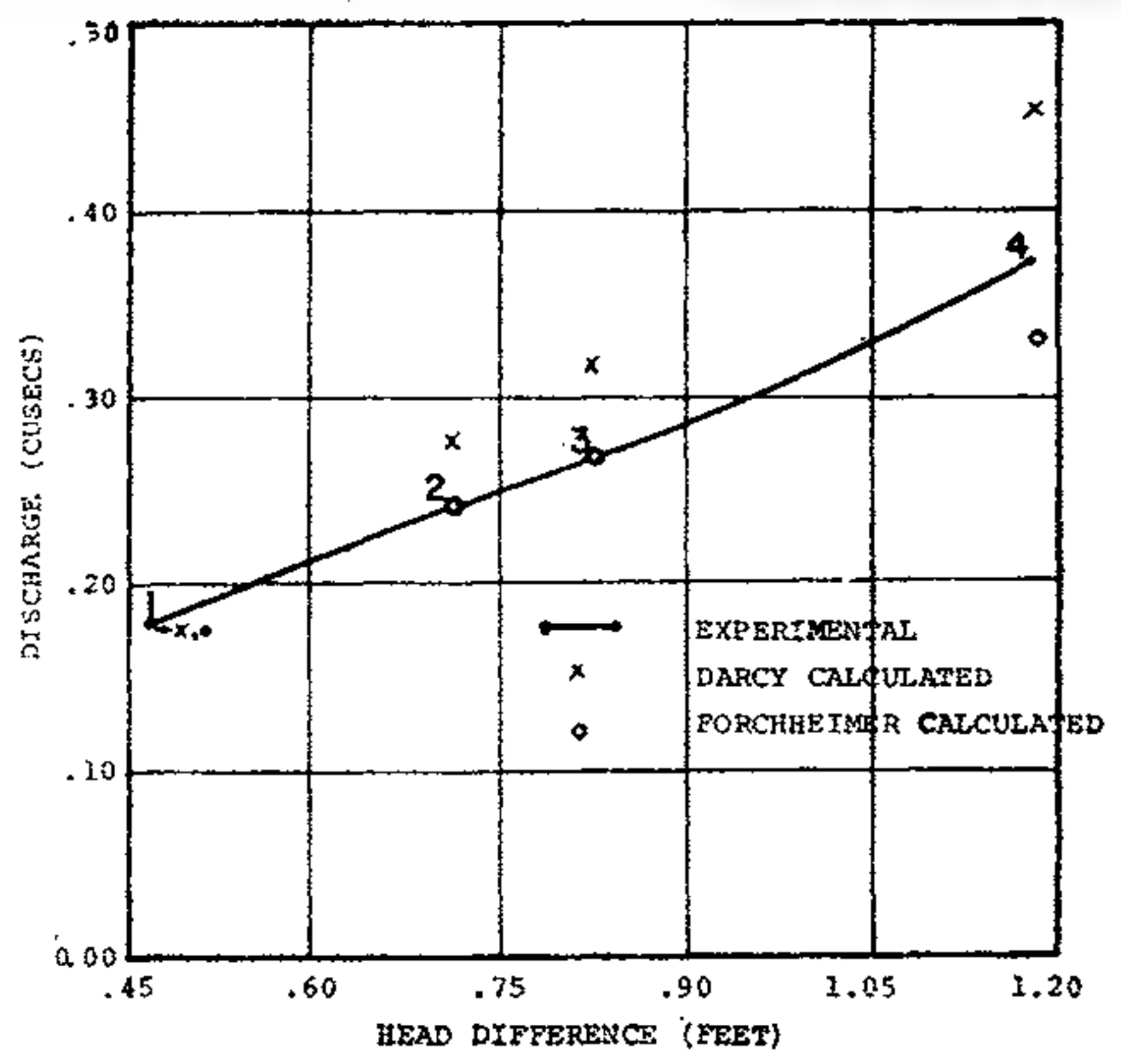
The velocities developed in flow No.3 have been estimated (Ref. 37) to have maximum values at the well interface of 0.15 ft./sec. compared with a velocity of 0.06 ft./sec. which was the maximum developed in the permeameter tests.
This velocity of 0.06 ft./sec. was also exceeded within a cylindrical column of radius 6 in. around the well.
When the flow was increased (flow No.4) to the condition where the velocity at the well interfacd was approximately 0.25 ft./sec. (i.e., four times the maximum permeameter velocity) and the excess region around the well was 8.5 in. radius then both the non-linear (Forchheimer) and the linear (Darcy) values were considerably in error, although the non-linear prediCtion was closer to the measured value.
This emphasises that whichever constitutive law is used predictive extrapolation beyond the range of actual test values is not generally warranted.
Other things being equal however the non-linear (Forchheimer) relationship is measurably superior to the Darcy equation.
Workers familiar with the problems of using the Darcy equation in practical situations frequently express the view that it is difficult enough to relate observed values of flow to a single variable-the Darcy coefficient of permeability, so that even greater difficulty is to be expected when dealing with a non-linear relationship such as the Forchheimer equation.
These experiments indicate the fundamental error encompassed in this opinion. In fact, it is much easier to relate the Forchheimer equation to actual flows now that the analytical difficulties inherent in handling non-linear equations have been overcome by the development of computer based numerical methods.
6.3 The Unconfined Aquifer:
Again, an axially symmetric situation was used with material similar to that described in section 6.2, i.e., fo in. nominal single size crushed granite aggregate. In this case both the Forchheimer and Missbach equations were used to predict the non-linear flow in a bed 5 ft. thick in the 20-ft. dia. tank.
Again, a reference flow (No.2) was used and the results are shown in Fig. 10. The superiority of both the non-linear expressions in this case is striking, the Darcy Law based predictions overestimating the maximum flow by 48%.
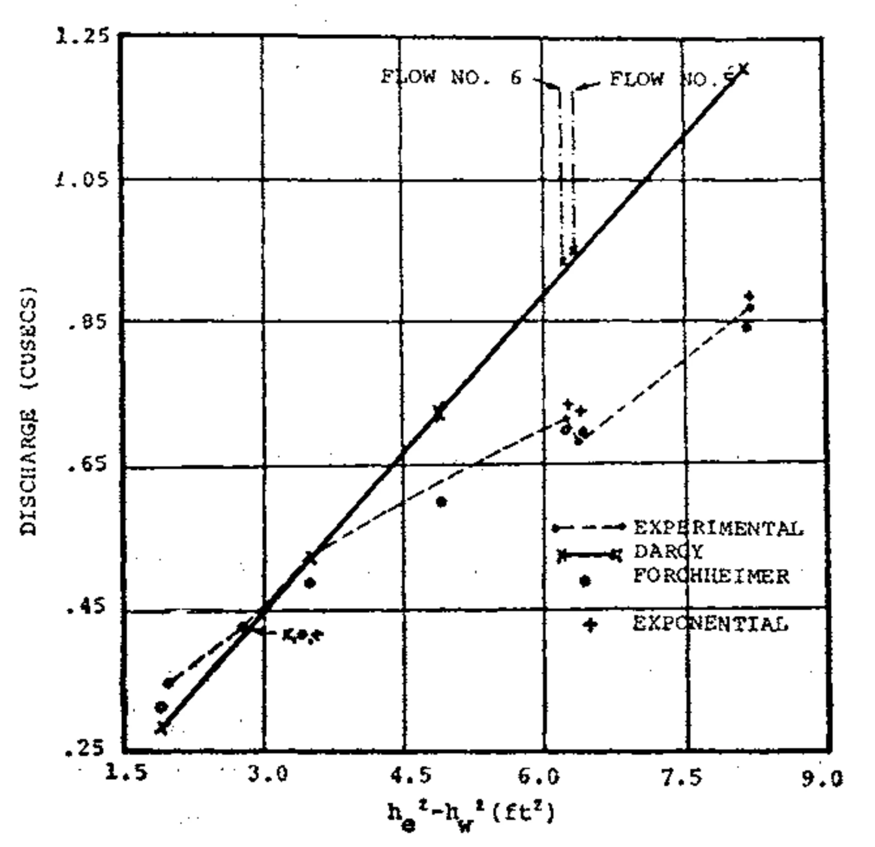
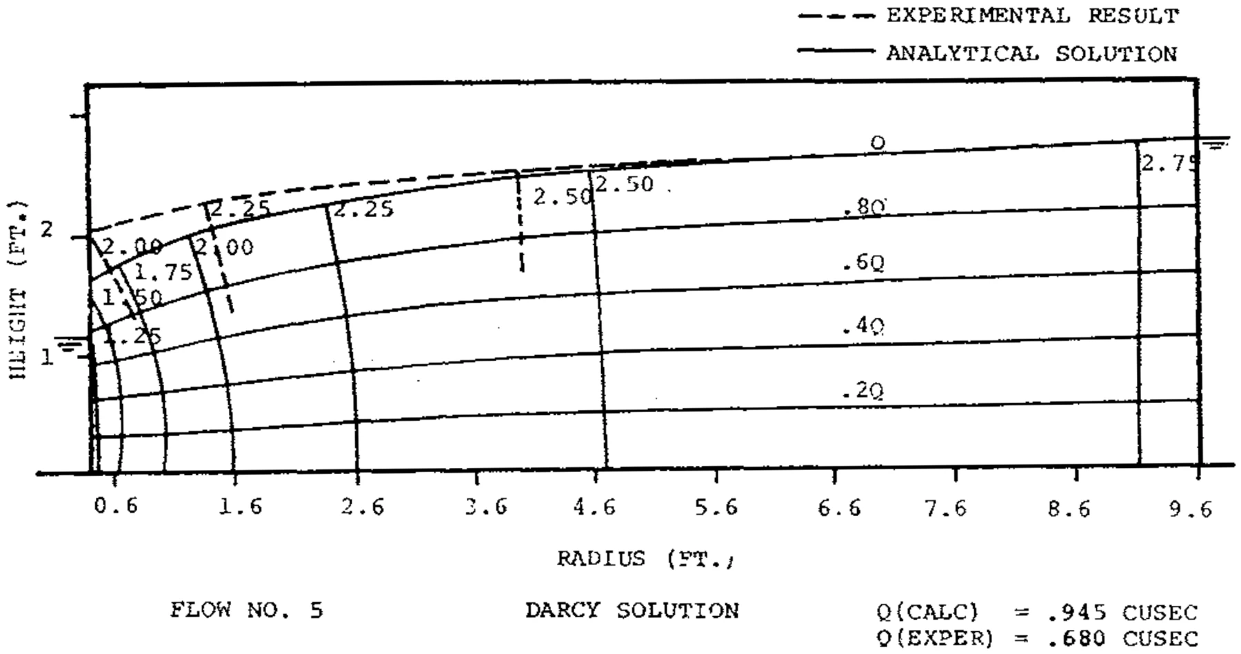
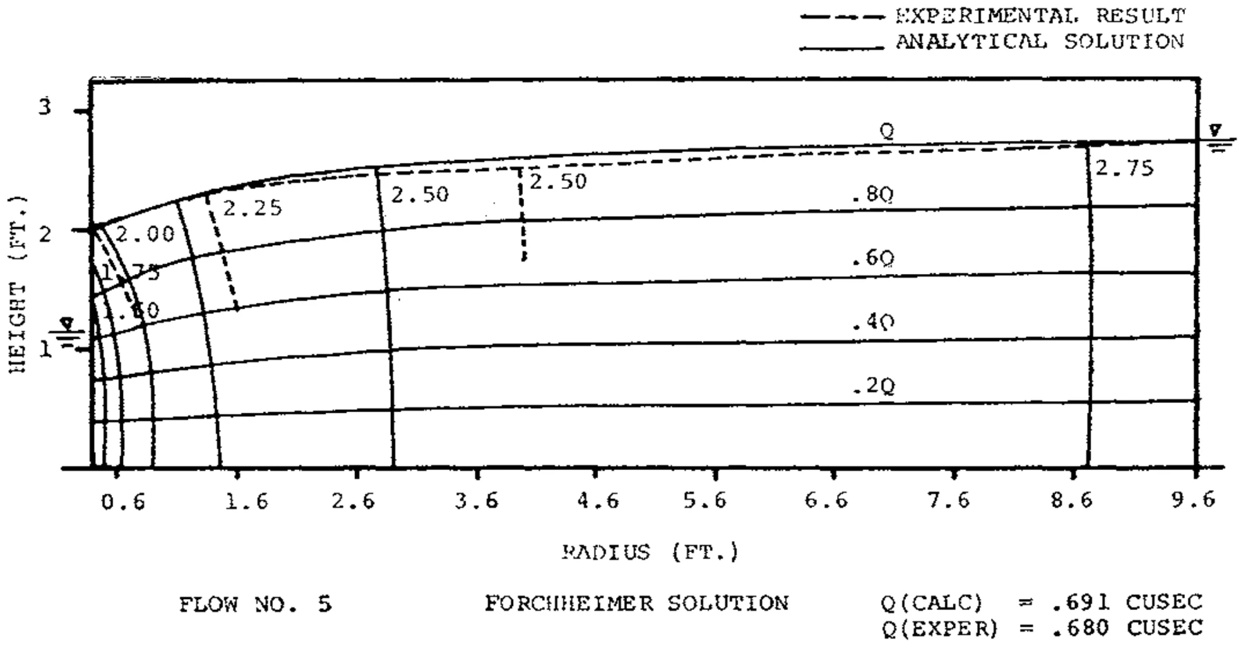
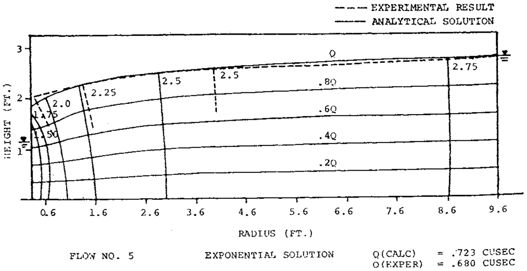
Figs. 11, 12 and 13 show a set of typical predicted flow nets at flow No.5. Again, although there is a significant difference between predicted and measured head differences with the non-linear equations, both are markedly superior to the Darcy Law based net.
6.4 Unconfined Flow Through a Permeable Wall:
In this case the aggregate was retained between two vertical sheets of metal gauze placed perpendicular to the direction of flow and approximately 3 ft. apart, thus simulating a simple two-dimensional cofferdam situation.
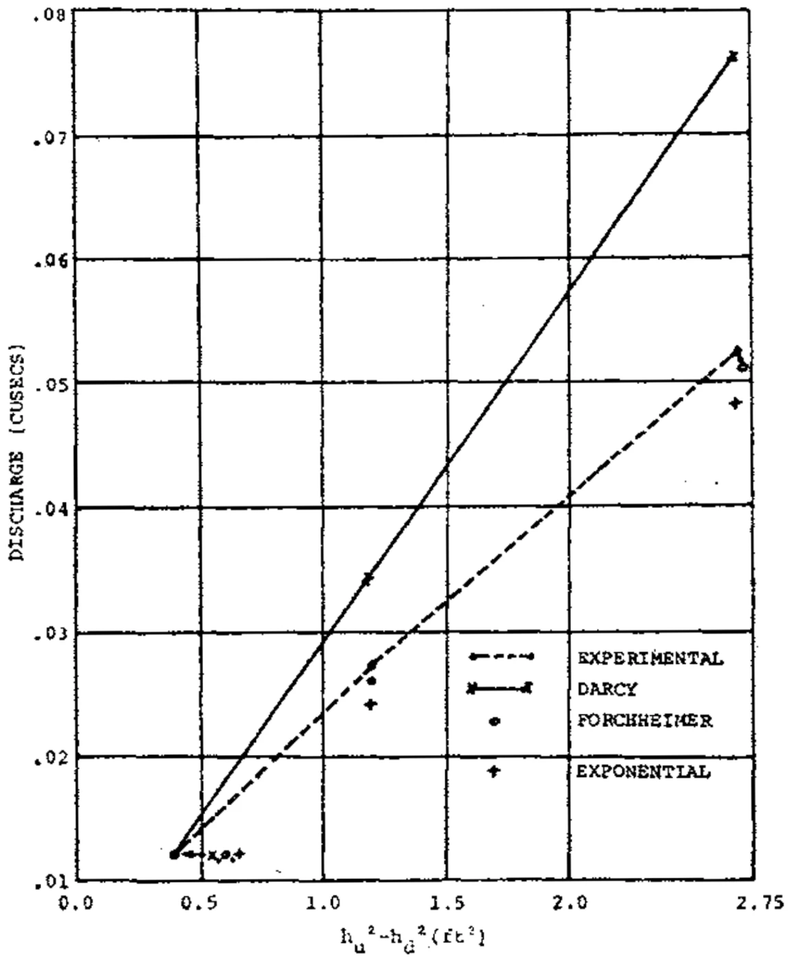
The results are shown in Fig. 14 and in this case the error involved in using Darcy’s Law is 46% whereas both non-linear predictions are within 1%.
6.5 Flow Through Model Dams:
Details of these experiments have been reported elsewhere (Ref. 36) but the resulting flow nets together with the relevant discharges are reproduced below for convenience (Fig. 15) .
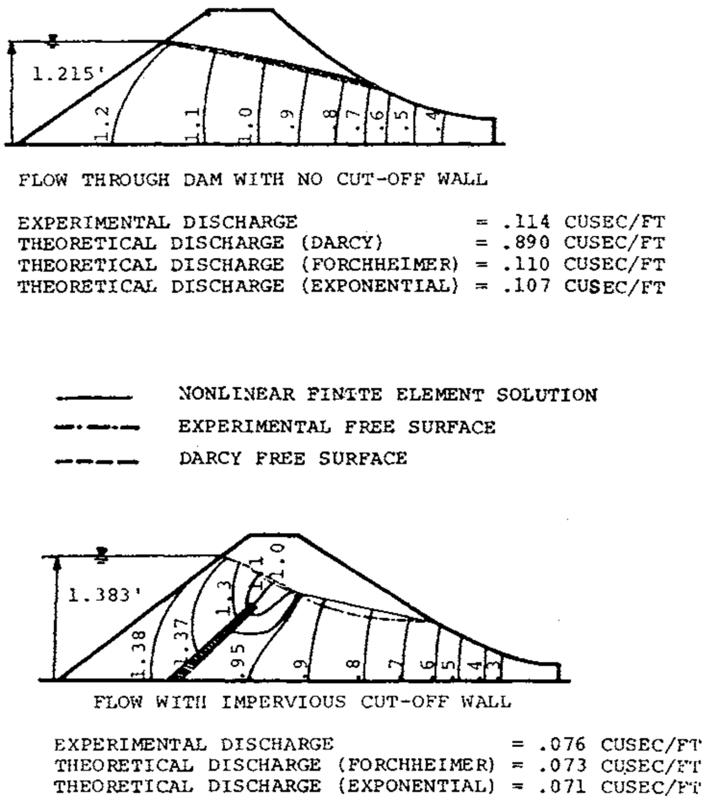
Again it will be evident that the non-linear equations give much better predictions than the Darcy equation with respect to discharge.
It is interesting to note however that there is little to choose between the methods as far as the prediction of the flow net is concerned. This is of considerable significance in relation to stability calculations.
Conclusions
Traditionally, analyses of flows in porous materials have been largely restricted to flows for which Darcy’s Law holds. There have been two reasons for this:
- flows through fine grained materials (less than 1 mm. average dimension) generally obey Darcy’s Law and
- analytical techniques for solving Laplace’s equation, which is the field equation for Darcy flow, are well developed and, indeed, analogous field relations hold in a number of other disciplines.
More recently it has become possible to investigate complex solutions of the Laplace equation using numerical techniques. Extension of these numerical procedures to solve more complex field equations has been a logical development so that it is now possible with very little additional effort (and possibly some additional computer time) to solve seepage problems which extend the basic head loss-flow relation well beyond the limits of validity of Darcy’s relation.
A natural step in this development has been to seek the most suitable and appropriate head loss-flow relation and although the literature abounds in empirical formulae it is interesting to note that a closer look at the fluid dynamics of porous media flow in terms of advanced numerical techniques has yielded a rational method of attack.
Flow through porous material can be viewed: (i) as a clastic problem and (ii) as a continuum problem. By considering the clastic problem it has been possible by integration to extend the basic flow relation within the power to a continuum relation which is representative of a given porous material and a given fluid.
It has been shown that under certain circumstances this relation reduces exactly to a Forchheimer relation whereas more generally the constants in the Forchheimer relation must be treated as variable. For certain idealised flows these variables can be accurately determined by numerical methods.
The rationale of the Forchheimer relation has been supported by a variety of experimental studies including a comprehensive series of tests using a parallel plate model-an extension of the Hele-Shaw apparatus.
Development of finite difference and finite element methods for solving the field equations resulting from a Forchheimer relation has been undertaken to illustrate that such problems present no serious difficulties to the present day engineer.
Finally the construction of a large scale experimental porous media tank has allowed the accuracy of these techniques to be checked against field conditions simulated in the laboratory. These tests have shown that serious errors in discharge estimation may be made if the Forchheimer relation is not used to replace Darcy’s equation and that the Forchheimer relation appears to give satisfactory results providing the appropriate coefficients are carefully determined.
Acknowledgments
The work described in this paper has been carried out in the Engineering laboratories at the James Cook University of North Queensland (formerly the University College of Townsville) and has been assisted financially from university funds.
The major financial support was provided by a series of grants from the Water Research Foundation of Australia Ltd. to whom the authors would express their appreciation.
Thanks are also due to Mrs. S. E. Hobson for assistance in typing and preparing the manuscript.
Appendix
(a) Three-Dimensional Derivation of Forchheimer Relation:
The three-dimensional Navier-Stokes equation in the x-direction for steady, incompressible flow is
and therefore
where , and , , . are vorticity components defined in the usual way.
Converting Eq. (A2) into dimensionless form as in Section 2.2 where gives
which can be compared with Eq. (13).
(b) Turbulent Flow—Two-Dimensional Derivation:
Note.— In this derivation bars over symbols are used to denote mean values with respect to time. Dimensionless quantities are distinguished by using the subscript as in .
If instantaneous velocities, e.g., are defined by where is the instantaneous variation from the mean then the two-dimensional equations for steady flow (Ref. 44) are given by
which can be rewritten as
where
and in dimensionless terms
which can be written in a Forchheimer format as for Eq. (A4) with modified coefficients.
References
- DARCY, H. — Les Fontaines Publiques de la Ville de Dijon. Paris, Victor Dalmont, 1856.
- SLICHTER, C.S. — Theoretical Investigation of the Motion of Groundwaters. U.S. Geol. Survey, 19th Annual Report, Part 2, 1897, p. 329.
- ADZUMI, H. — The Flow of Gases through Metallic Capillaries at Low Pressures. Bulletin Chem. Soc. Japan, 1939, pp. 343-7.
- CHILDS, E.C. and COLLIS-GEORGE, N. — The Permeability of Porous Materials. Proc. Roy. Soc., Series A, Vol. 201, No. 1066, May 23, 1950, pp. 392-405.
- MARSHALL, T.J. — Permeability Equations and Their Models. Proc. Symposium on Interaction between Fluids and Particles. London, Adlard, 1962, pp. 299-303.
- KOZENY, J. — Soil Permeability. Wassers in Boden Setz-Ber. Wiener Akad., Vol. 136, 1927, pp. 271-306.
- CARMAN, P.C. — Fluid Flow through Granular Beds. Trans. I. Chem. E., Vol. 15, 1937, pp. 150-66.
- WYLLIE, M.R.J. and GREGORY, A.R. — Gulf Research and Development Co., Pittsburgh, Geol. Div., Report No. 41, 1954.
- HUBBERT, M.K. — Darcy’s Law and the Field Equations of Flow of Underground Fluids. Jour. Petrol. Technology, Vol. 8, 1956, pp. 222-39.
- FORCHHEIMER, P.H. — Hydraulik. Berlin, Teubner, 1930.
- ARAVIN, B.I. and NUMEROV, S.N. — Theory of Fluid Flow in Undeformable Porous Media. Jerusalem, Israel Program for Scientific Translations, 1965.
- WARD, J.C. — Turbulent Flow in Porous Media. Proc. A.S.C.E., Jour. Hydraulic Div., Vol. 90, No. HY5, Sept., 1964, pp. 1-12.
- LINDQUIST, E. — On the Flow of Water through Porous Soil. Trans. First Congress on Large Dams, Stockholm, 1933, Vol. 5, pp. 81-101.
- IRMAY, S. — On the Theoretical Derivation of Darcy and Forchheimer Formulas. Trans. Amer. Geophys. Union, Vol. 39, 1958, pp. 702-7.
- MISSBACH, A. — Listy Cukrova, Vol. 55, 1937, p. 293.
- WHITE, A.M. — Pressure Drop and Loading Velocities in Packed Towers. Chem. Engg. Progress, Vol. 31, 1935, pp. 390-408.
- ESCANDE, L. — Experiments Concerning the Infiltration of Water through a Rock Mass. Proc. Minnesota Int. Hydraulics Convention, Minneapolis, 1953, pp. 547-53.
- WILKINS, J.K. — The Flow of Water through Rockfill and its Application to the Design of Dams. Proc. Second Aust.-New Zealand Conf· Soil Mechanics and Foundation Engg., Christchurch, 1956, pp. 141-7.
- PARKIN, A.K., TROLLOPE, D.H. and LAWSON, J.D. — Rockfill Structures Subject to Water Flow. Proc. A.S.C.E., Jour. Soil Mechanics and Foundations Div., Vol. 92, No. SM6, Nov., 1966, pp. 135-51.
- ANANDAKRISHNAN, M. and VARADARAJULU, G.H. — Laminar and Turbulent Flow of Water through sand. Proc. A.S.C.E.; Jour. Soil Mechanics and Foundations Div., Vol. 89, No. SM5, Sept., 1963, pp. 1-15.
- DUDGEON, C.R. — Flow of Water through Coarse Granular Materials. Thesis (M.E.), University of New South Wales, 1964.
- WATSON, K.K. — The Permeability of an Idealised Two-Dimensional Porous Medium using the Navier-Stokes Equations. Proc. Fourth Aust.-New Zealand Conj. Soil Mechanics and Foundation Engg., Adelaide, 1963, pp. 37-40.
- PHILIP, J.R. — Fluid Flow in Porous Media from the Viewpoint of Classical Hydrodynamics. Proc. Second Aust. Conf. Soil Science, 1957, Vol. 1, pp. 1-9.
- TROLLOPE, D.H. — The Mechanics of Discontinua or Clastic Mechanics in Rock Problems. Chapter 9 of Rock Mechanics in Engineering Practice. Edited by Stagg, K.G. and Zienkiewicz, O.C. London, Wiley, 1968.
- SCHLICHTING, H. — Boundary Layer Theory. New York, McGraw-Hill,1960.
- STARK, K.P. — Some Aspects of the Non-linear Laminar Regime of Flow in Porous Media. Thesis (Ph.D.), University of Queensland, 1968.
- STARK, K.P. — A Numerical Study of the Non-linear Laminar Regime of Flow in an Idealized Porous Medium. Proc. I.A.H.R. Symposium, on “The Phenomena in Porous Media“, Haifa, Feb., 1969.
- TEK, M.R. — Development of a Generalised Darcy Equation. Trans. A.I.M.M.E., Vol. 210, 1957, pp. 376-8.
- ROSE, H.E. — Fluid Flow through Beds of Granular Material. Some Aspects of Fluid Flow. London, Edward Arnold, 1951, pp. 136-62.
- GUNN, D.J. and MALIK, A.A. — Flow through Expanded Beds of Solids. Trans. I. Chern. E., Vol. 44, 1966, pp. T371-87.
- HOW LUM, C. — An Investigation into Porous Media Flow. Thesis (B.E.), University College, Townsville, 1966.
- STARK, K.P. and VOLKER, R.E. — Non-linear Flow through Porous Materials-Some Theoretical Aspects. University College, Townsville, Dept. of Engg., Research Bulletin No. 1, 1967.
- VOLKER, R.E. — Flow through Idealized Particle Arrays. Thesis (M.Eng.Sc.), University College, Townsville, 1966.
- KRISTIANOVICH, S.A. — Movement of Groundwaters Violating Darcy’s Law. Jour. Applied Math. and Mechanics, Vol. 4, 1940, pp. 33-52.
- ENGELUND, F. — On the Laminar and Turbulent Flows of Groundwatter through Homogeneous Sand. Tech. University of Denmark, Hydraulic Labs., Bulletin No.4, 1953.
- VOLKER, R.E. — Non-linear Flow in Porous Media by Finite Elements. Proc. A.S.C.E. Jour. Hydraulic Div., Vol. 95, No. HY6, Nov., 1969, pp. 2093-114.
- VOLKER, R.E. — Numerical Solutions to Problems of Non-linear Flow through Porous Materials. Thesis (Ph.D.), James Cook University of North Queensland, 1969.
- BOULTON, N.S. — The Flow Pattern near a Gravity Well in a Uniform Water Bearing Medium. Proc. I.C.E. Vol. 36, 1950-51, pp. 534-50.
- COURANT, R. and HILBERT, D. — Methods of Mathematical Physics. Vol. 1. New York, Interscience Publications, 1953.
- ZIENKIEWICZ, O.C. and CHEUNG, Y.K. — Finite Elements in the Solution of Field Problems. The Engineer, Vol. 220, No. 5722, Sept. 24th, 1965, pp. 507-10.
- PARS, L.A. — An Introduction to the Calculus of Variations. London, Heinemann, 1962.
- FENTON, J.D. — Hydraulic and Stability Analyses of Rockfill Dams. University of Melbourne, Dept. of Civil Engg., Report No. DR15, 1968.
- PARKIN, A.K. — Rockfill Dams with Inbuilt Spillways, Part I – Hydraulic Characteristics. Water Research Foundation of Aust. Bulletin No.6, 1963.
- HINZE, J.O. — Turbulence. New York, McGraw-Hill, 1959.