An evaluation of empirical correlations for the compression and swell indices for Queensland soil conditions

B.G. Look and D.J. Williams

Abstract

Empirical relationships for the compression and swell indices of soils are used extensively in preliminary design studies. This forms the basis to determine the suitability of a site or the thrust for further testing of that site. The intent of this paper is to evaluate existing relationships found in the literature for these soil indices and to assess which of the many relationships provide a reliable correlation for Queensland soil conditions. The review indicates that the indices are better related to moisture content than to liquid limit and the strength of the relationship varies, depending on the stress history of the soil.

1. Introduction

The compression index $C_c$ and the swelling index $C_s$ are often used in the calculation of clay foundation movements. Figure 1 shows a typical void ratio vs. $Log_{10}$ pressure plot and defines $C_c$ as the slope of the straight line portion of the loading curve on the virgin consolidation line, while $C_s$ is the slope of the unloading curve. These parameters are defined by Eqs. 1 and 2.

Virgin Compression Line

\begin{equation} C_c = {de \over d(Log p)} \label{eq:virgin} \end{equation} \ref{eq:virgin} (Eq. 1)

Swelling Line

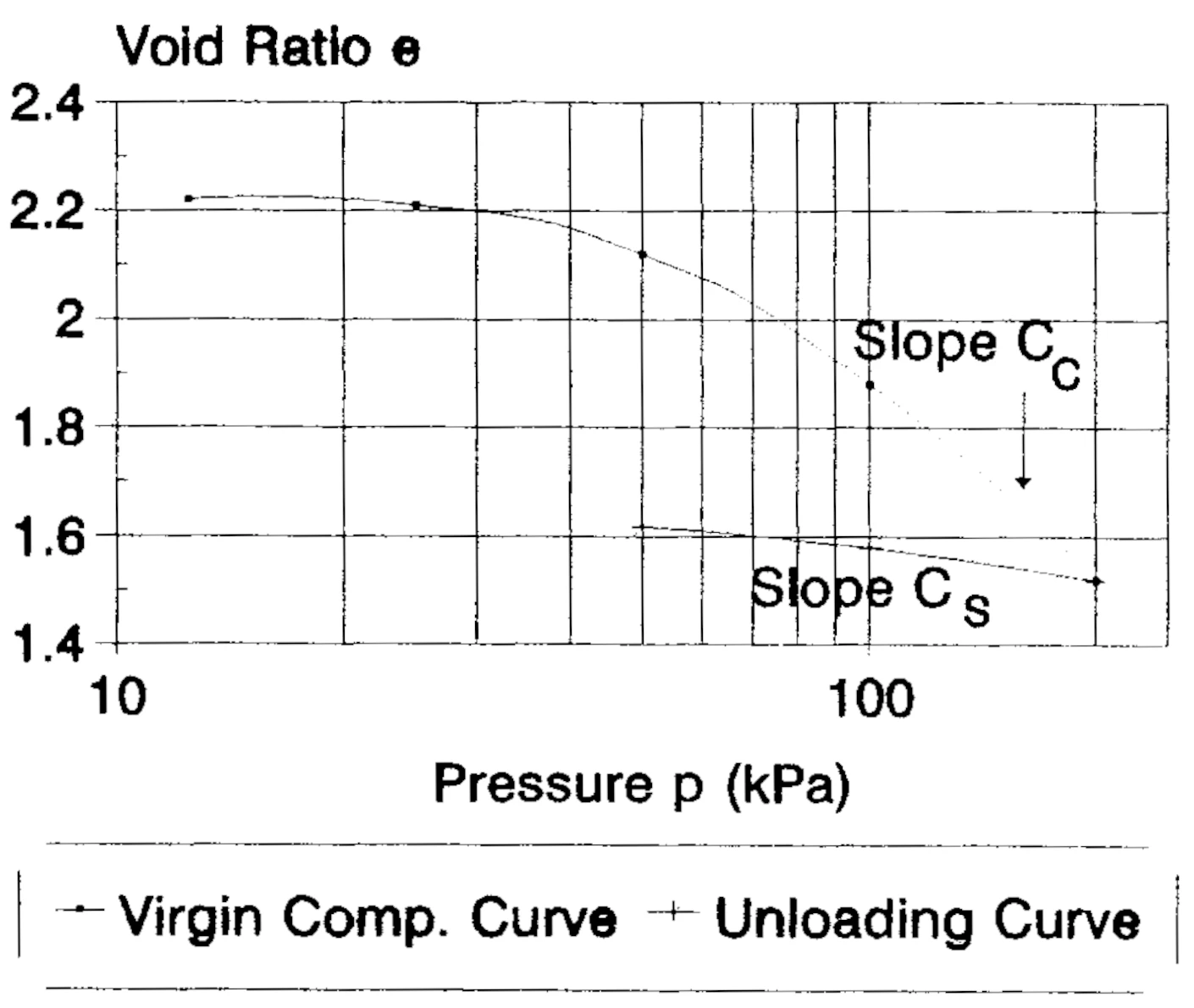
\begin{equation} C_s = {de \over d(Log p)} \label{eq:swell} \end{equation} \ref{eq:swell} (Eq.2)

The choice between the compression and swell indices in the calculation of consolidation settlement Sc depends on the stress history of the soil (Eqs. 3,4,5). The stress history is based on the ratio of the preconsolidation pressure $p_c$ to the existing overburden pressure $p_o$ . The former separates the behaviour of the soil from predominantly elastic (represented by $C_s$ ) to mainly plastic (represented by $C_c$ )·

\begin{equation} S_c = {{C_c\ H_c} \over 1 + e_o}\ Log\ {{P_o + \delta p_{av}} \over p_o} \label{eq:3} \end{equation} \ref{eq:3} (Eq. 3)

(normally consolidated clays with $P_o > P_c$ )

\begin{equation} S_c = {{C_s\ H_c} \over 1 + e_o}\ Log\ {{P_o + \delta p_{av}} \over p_o} \label{eq:4} \end{equation} \ref{eq:4} (Eq. 4)

(overconsolidated soils with $p_o+\delta p_{av}<p_c$ )

\begin{equation} S_c = {{C_s\ H_c} \over 1 + e_o}\ Log\ {p_c \over p_o}+{{C_c\ H_c} \over 1 + e_o}\ Log\ {{p_o + \delta p_{av}} \over p_c} \label{eq:5} \end{equation} \ref{eq:5} (Eq. 5)

(overconsolidated soils with $p_o < p_c<p_o+ \delta p_{av}$ )

Use of the coefficient of volume compressibility my is often preferred to the use of $C_c$ and $C_s$ (Wesley, 1987) because it represents a strain-stress relationship which provides a more direct formula for settlement calculation. The relationship is defined in Eq. 6 and the calculation of $S_c$ follows from Eq. 7.

\begin{equation} m_v = {\delta \epsilon \over \delta p} = \Bigg( {{e_o – e_1} \over {1 + e_o}} \Bigg) {1 \over {p_1 – p_o}} = {S_c \over H}\ {1 \over \delta p} \label{eq:6} \end{equation} \ref{eq:6} (Eq. 6)

\begin{equation} S_c = m_v \ H \ \delta p \label{eq:7} \end{equation} \ref{eg:7}(Eq. 7)

In preliminary design and to supplement consolidation test results, empirical relationships are often used to estimate the compression and swell indices. The coefficient of volume compressibility is not a fundamental parameter since it is based on the applied stress and therefore _empirical relationships with other parameters have not been established.

The existing empirical relationships relate the compression index to the liquid limit, natural moisture content or initial void ratio of the soil. The validity of these relationships are discussed in this paper.

The unloading (swelling) line for overconsolidated soils may be used to calculate heave in expansive clay sites by using Eqs. 8 and 9 (a variation of Eq. 4).

\begin{equation} \text{Total Heave } \Delta h_i = \Sigma h_i \label{eq:8} \end{equation} \ref{eq:8} (Eq. 8)

\begin{equation} \Delta h_i = h_i \ { C_s \over 1 + e_o}\ Log\ {p_f \over p_c} \label{eq:9} \end{equation} \ref{eq:9} (Eq. 9)

$p_f$ = Final stress state
$p_o$ = Initial stress state

In this regard, the value of $C_s$ is given as 114 (25%) to 115 (20%) of $C_c$ (Das, 1984) and 5 to 10% of $C_c$ (Carter and Bentley, 1991). The validity of these relationships is also discussed in this paper.

2. Sources of data

Data for analysis was obtained from reports filed at the Materials and Geotechnical Services Branch, Queensland Department of Transport (QT) which included both consultant’s and internal reports.

In many instances there was some variability in reporting style and some parameters had to be calculated. The degree of overconsolidation was also calculated for each sample. A total of 87 data points were tabled from the QT data source for analysis.

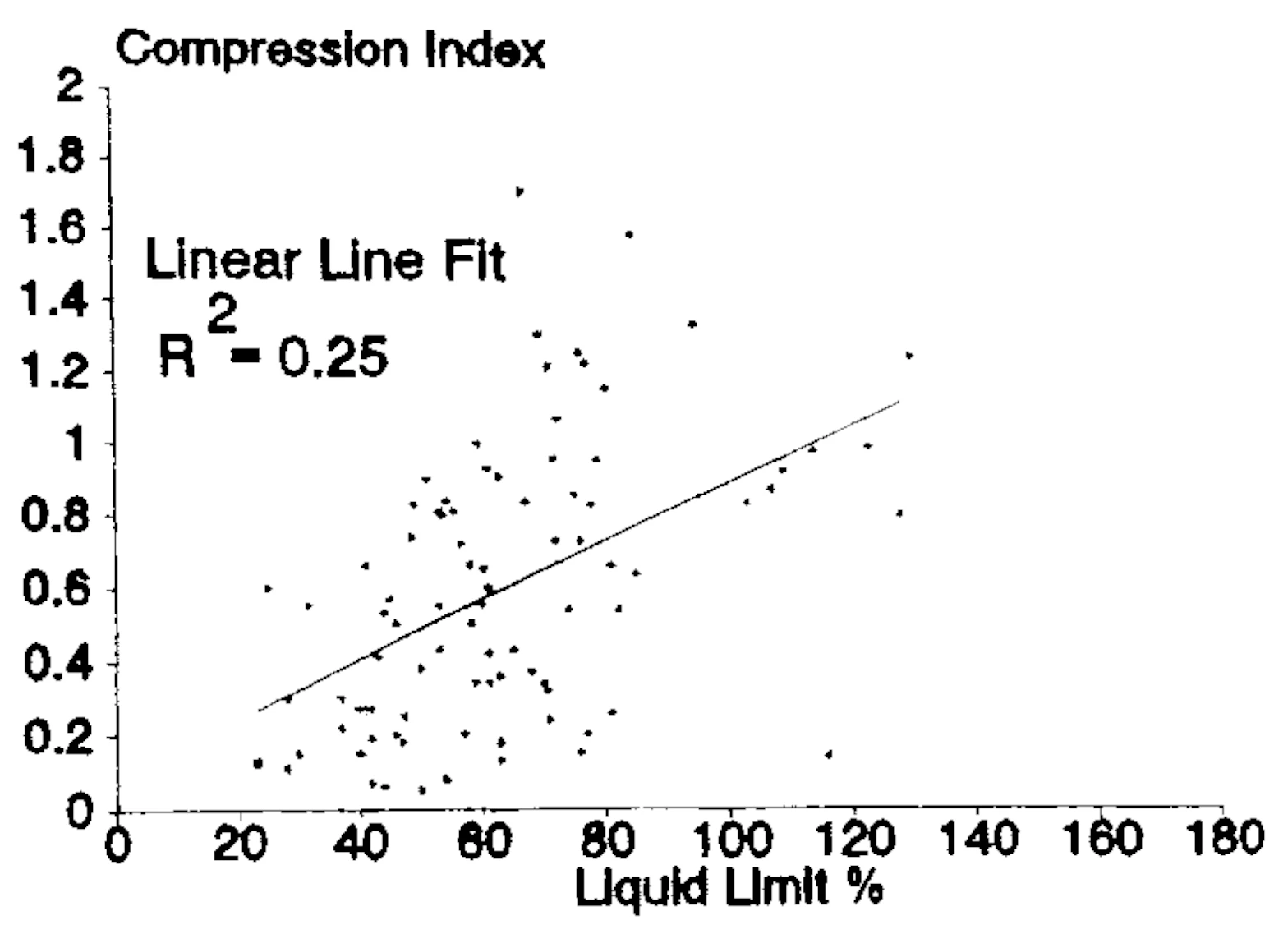
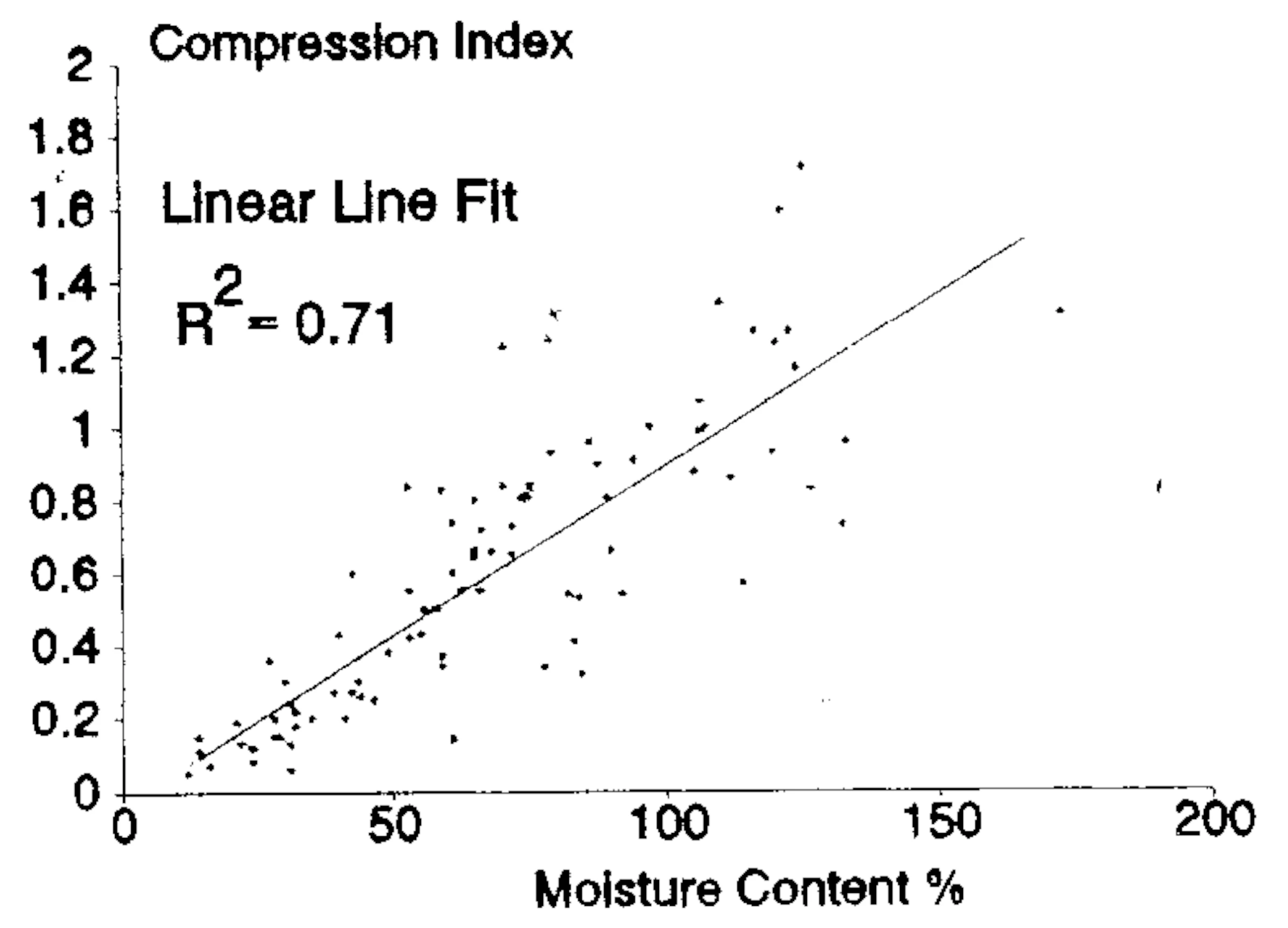
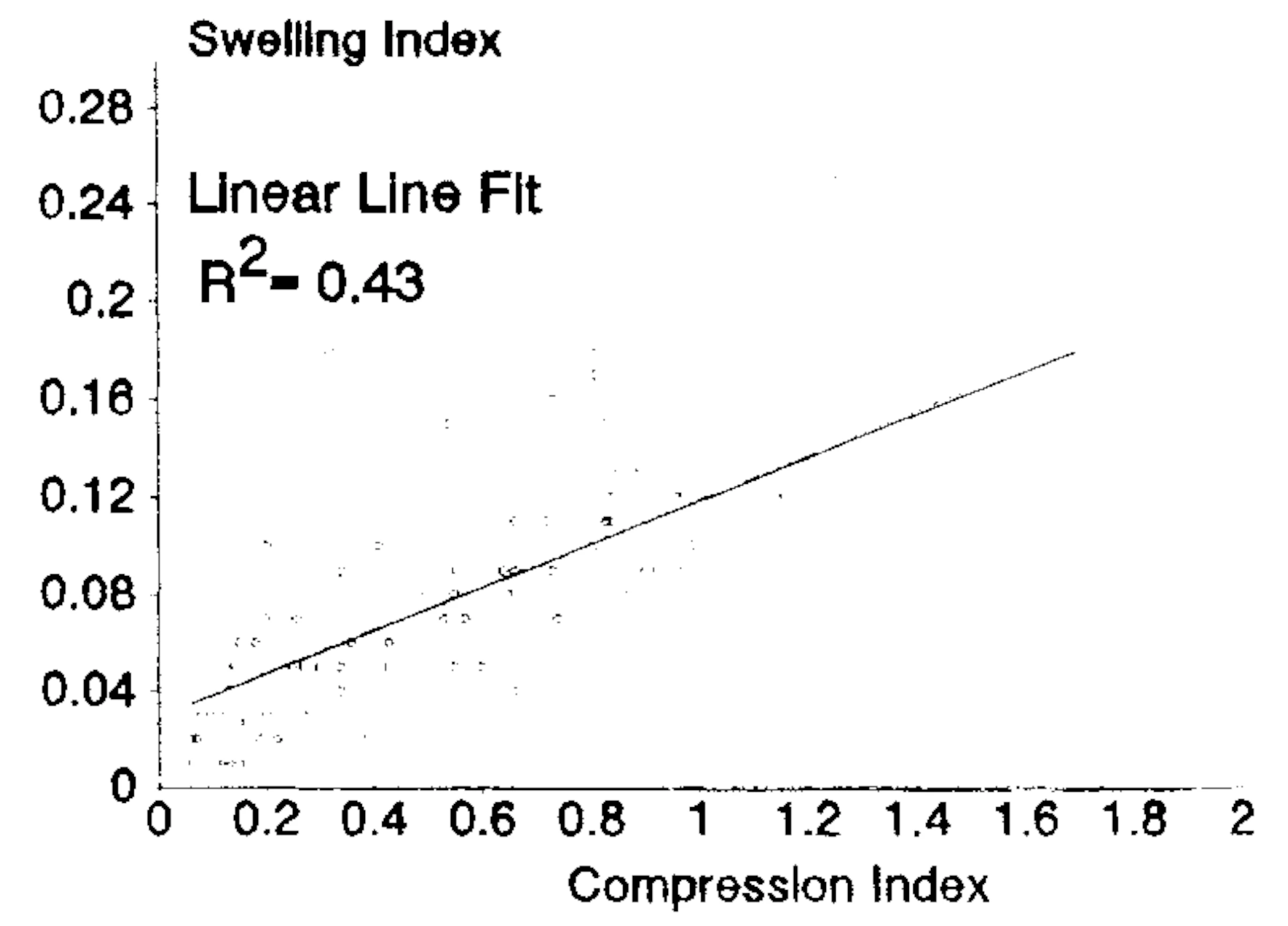
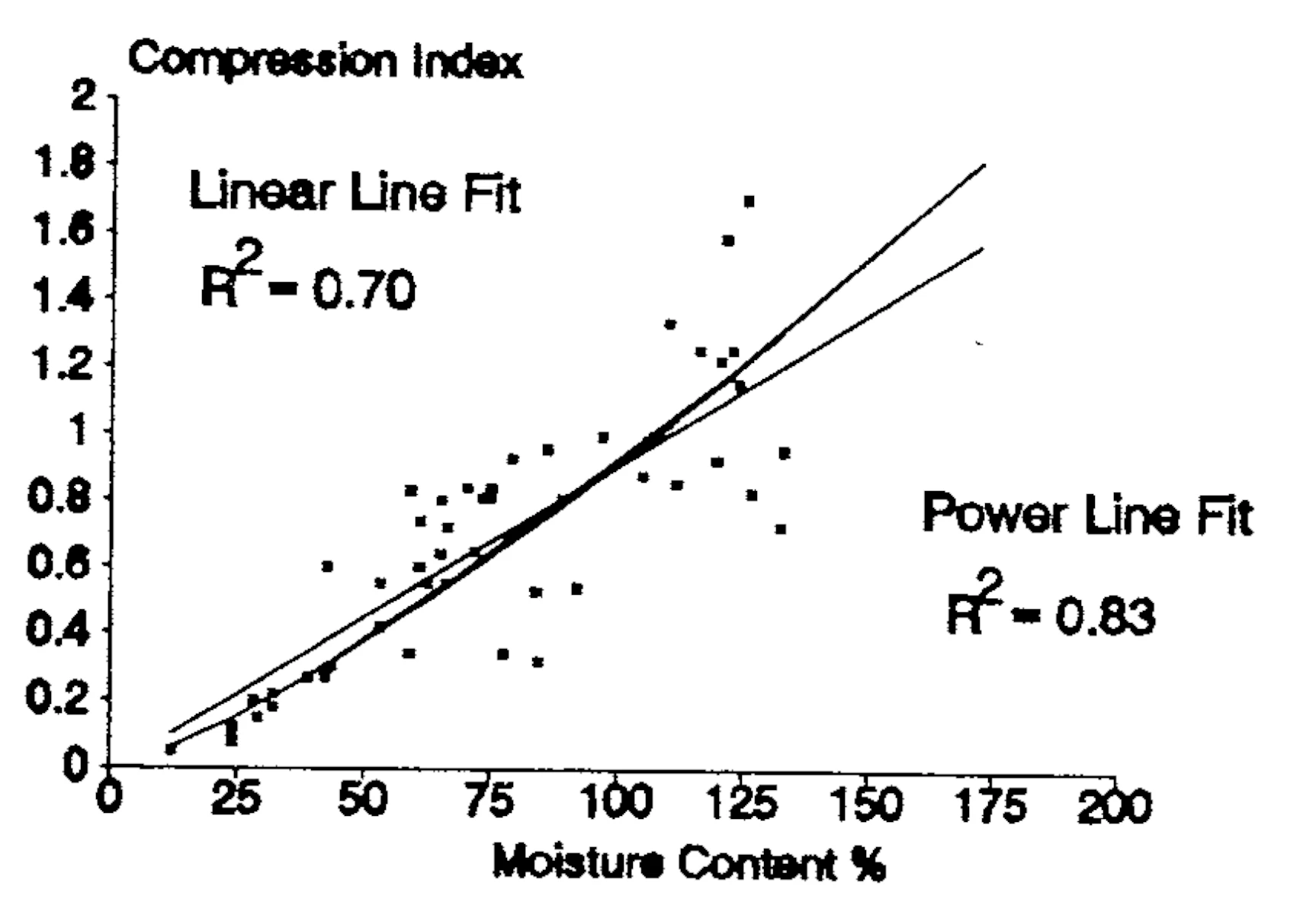
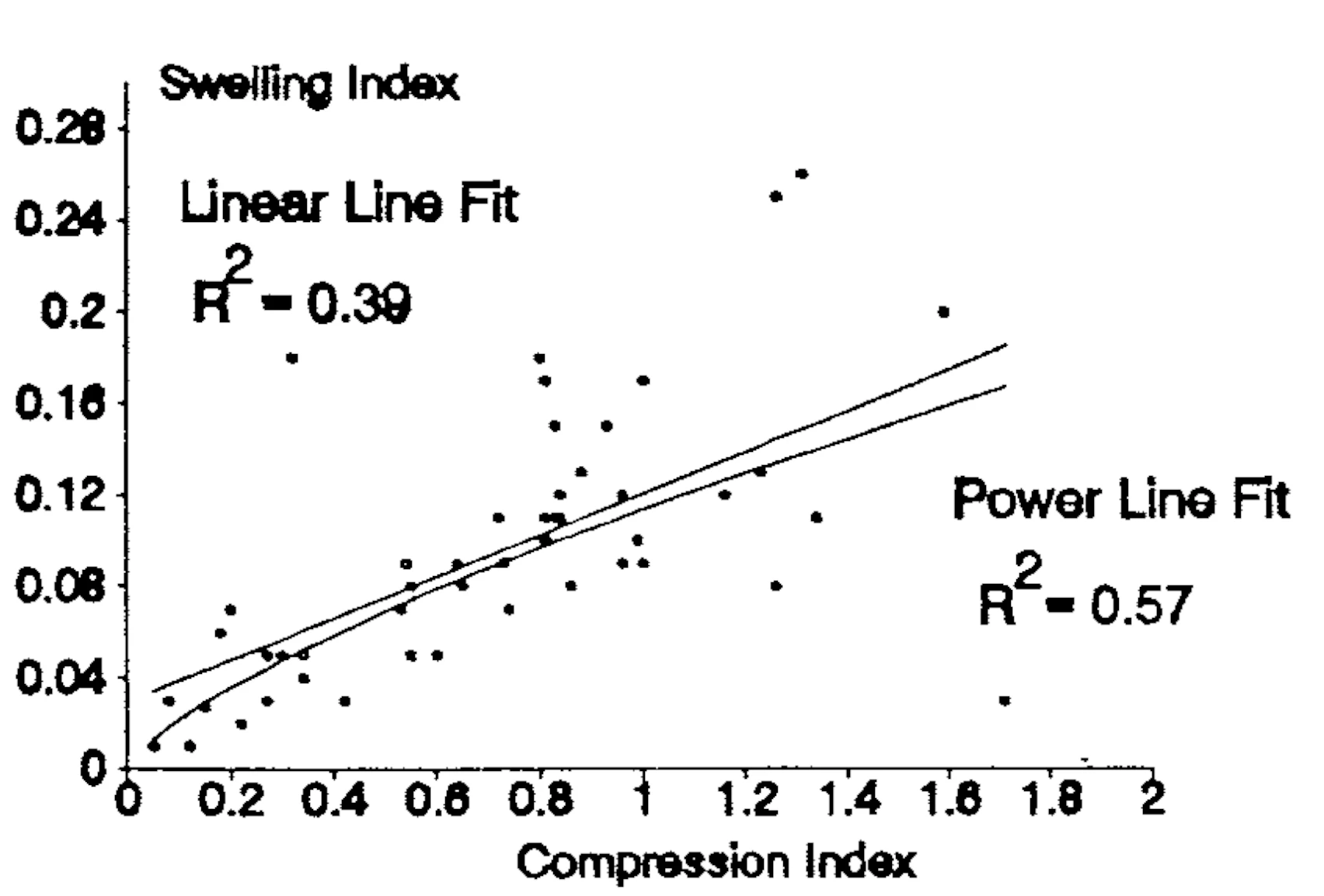
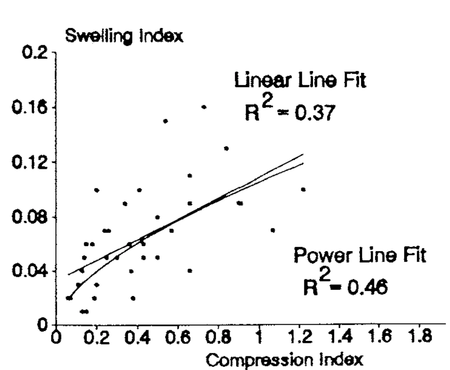
The data points are shown in Figures 2, 3 and 4 together with the linear regression lines.

Figure 2: Relationship between compression index and liquid limit

Figure 3: Relationship between compression index and moisture content

Figure 4: Relationship between swell index and compression index

3. Existing correlations

Selected empirical relationships between $C_c$ and liquid limit $LL$ or natural moisture content $w_n$ are given in Table 1. Terzaghi and Peck (1948) modified Skempton’s (1944) relationship between $C_c$ and $LL$ for remoulded clays. Bowles (1979) provided a similar relationship for Brazilian Clays, but with different constants.

Reference	$C_c$ Relationship	Regions of applicability
Skempton (1944)	$.009\ (LL – 10)$	Normally consolidated clays
Terzaghi and Peck (1948)	$.007\ (LL – 10)$	Remoulded clays
Bowles (1979)	$.0046\ (LL – 9)$	Brazilian clays (D.C.)
Koppula (1981)	$.01\ w_n$	Chicago clays (N.C.)
Bowles (1979)	$.0115\ w_n$	Organic silts and clays

Table 1: Empirical equations from the literature

Other authors have also established relationships between $C_c$ and $LL$ . These have been summarised by Azzouz et al. (1976) and also evaluated by Nagaraj and Murphy (1986).

While relationships of the form given in Table 1 are often accepted, calibration against local conditions is required before they can be applied. This paper attempts to calibrate these relationships for Queensland soil conditions.

4. Analysis of Queensland Data

The following regression relationships were fitted to the QT data.

1. Linear	$Y = a + b\ X$
2. Logarithm	$Y = a + b\ Ln\ X$
3. Exponent	$Y = a\ c^{b\ X}$
4. Power	$Y = a\ X^b$

The constants, a and b, and correlation coefficient $R^2$ obtained for these regression relationships are given in Table 2.

Table 2 shows that for the $C_c$ vs $LL$ relationship, a linear fit relationship (25% of the variation explained) would be the best overall, representing a moderate to weak correlation. The minor improvement in the $R^2$ value for the logarithmic relationship does not justify its usage considering the simplicity of the linear relationship.

For the $C_c$ vs $w_n$ relationship all types of regression provide a good fit, with the linear fit explaining 71% of the variation. The power line law provides the best account of the variation, with 78% of the values explained.

Relationship	Type	$a$	$b$	$R^2$
$C_c \text{ vs }LL$	Linear	0.078	0.008	0.25
	Log			0.26
	Exp			0.21
	Power			0.24
$C_c \text{ vs } w_n$	Linear	-0.038	0.009	0.71
	Log			0.67
	Exp			0.68
	Power	-5.741	1.218	0.78
$C_s \text{ vs } C_c$	Linear	0.030	0.089	0.43
	Log			0.43
	Exp			0.43
	Power	-2.194	0.667	0.55

Table 2: Regression relationships for QT data

The $C_s$ vs $C_c$ relationship was also best represented by a power law fit with 55% of the variation explained, compared with 43% for the linear fit.

The relationship between $C_c$ and $LL$ or moisture content ( $w_n$ ) were compared with those determined for Brisbane soils by Strohfeldt (1991), which used data different to the data source used herein.

Strohfeldt’s data with 110 observation points was reanalysed separately in expectation of similar trends. As shown in Table 3, these expressions were only partly realised with the linear fit being the best for the $C_s$ vs $LL$ and $C_c$ vs $w_n$ relationships. Lower correlation coefficients were obtained with slightly different regression lines. Analysis of the two separate data sets both show w n providing a better correlation with $C_s$ than $LL$ .

Relationship	Type	$a$	$b$	$R^2$
$C_c \text{ vs }LL$	Linear	-0.063	0.007	0.18
	Log	-1.184	0.378	0.18
	Exp			0.16
	Power			0.17
$C_c \text{ vs } w_n$	Linear	-0.122	0.009	0.31
	Log			0.22
	Exp			0.23
	Power			0.19

Table 3: Regression relationships for Strohfeldt’s data

Two possible reasons for the discrepancy between the two sources of data could be the following:

A bias based on the degree of overconsolidation of the soils analysed with Strohfeldt’s data covering a broader range of soil types than the predominantly normally consolidated QT data.
Different quality testing from the various sources.

Table 4 shows that the QT data represent a more compressible soil. This data was separated into normally consolidated and overconsolidated clays for further regression analysis.

Source of data set	No. of points	$C_c$	$LL$	$w_n$
Strohfeldt	110	.35	61.0	50.3
QLD Transport	87	.60	63.3	68.0

Table 4: Data summaries

Table 5 shows the results of linear regression analysis on the normally consolidated NC and overconsolidated OC QT data compared with that carried out on the combined data set.

Soil (No. of points)	Index	$R^2$
Soil (No. of points)	Index	$w_n$	$LL$	$w_n \text{ \& } LL$	$C_c$
All (87)	$C_c$	0.71	0.25	0.71	–
All (87)	$C_s$	0.43	0.36	0.51	0.43
NC (36)	$C_c$	0.70	0.29	0.70	–
NC (36)	$C_s$	0.41	0.37	0.49	0.39
OC (51)	$C_c$	0.59	0.06	0.59	–
OC (51)	$C_s$	0.31	0.23	0.41	0.37

Table 5: Linear correlations for QT data

The results in Table 5 indicate the following:

Overall for all clays a strong linear relationship between $C_c$ and $w_n$ was found.
For overconsolidated clays the relationship between $C_c$ or $C_s$ and $LL$ is weak.
A multiple regression of $C_c$ with $LL$ and $w_n$ does not improve the correlation.
A multiple regression of $C_s$ with $LL$ and $w_n$ improves the correlation.
$C_s$ is more strongly related with $LL$ than with $C_c$ .
The relationship between $C_c$ and $C_s$ shows similar strength irrespective of the state of the clay.
For overconsolidated clays, the relationship between $w_n$ (rather than $LL$ ) should be used.

Analysis using the non-linear regression types on the same data was also carried out, and the full results are given in Tables 6 and 7.

Relationship	Type	$a$	$b$	$R_2$
$C_c \text{ vs }LL$	Linear	-0.152	0.008	0.29
	Log	-1.667	0.576	0.32
	Exp			0.26
	Power			0.29
$C_s \text{ vs }LL$	Linear	-0.002	0.001	0.37
	Log			0.36
	Exp			0.37
	Power	-7.585	1.212	0.41
$C_c \text{ vs } w_n$	Linear	-0.010	0.009	0.70
	Log			0.69
	Exp			0.66
	Power	-5.948	1.272	0.83
$C_s \text{ vs } w_n$	Linear	0.013	0.001	0.41
	Log			0.41
	Exp			0.45
	Power	-6.835	1.005	0.57
$C_s \text{ vs } C_c$	Linear	0.030	0.091	0.39
	Log			0.39
	Exp			0.42
	Power	-2.174	0.718	0.57

Table 6. Regression relationships for normally consolidated clays (51 QT data points)

The results in Tables 6 and 7 show that the power law fit explains more of the data variability in most cases. Selected power law fits are plotted together with the linear fits in Figures 5 to 7 and it can be seen that the fringe points (at the end of the curve/line) strongly influence whether a linear or non-linear relationship is stronger. Therefore, it is questionable whether the gains of using the power law fits, with its stronger relationship, can be justified given the reliability of the fringe points and the simplicity of linear relationships.

Table 8 provides a general summary of the linear relationships for the Queensland clays analysed. Comparing the result in Table 8 with the relationship in Table 1, indicate the following.

The regression constants for Queensland soils are different from those quoted in the literature.
The ratio of $C_s$ to $C_c$ is 9% and 8% for NC and OC clays respectively based on QT data. This is within the 5 to 10% range quoted by Carter and Bentley (1991), but outside the 20 to 25% range quoted by Das (1984).

Relationship	Type	$a$	$b$	$R_2$
$C_c \text{ vs }LL$	Linear	-0.192	0.004	0.06
	Log			0.10
	Exp			0.07
	Power	-4.187	0.767	0.12
$C_s \text{ vs }LL$	Linear	0.010	0.001	0.23
	Log			0.28
	Exp			0.31
	Power	-7.994	1.267	0.40
$C_c \text{ vs } w_n$	Linear	-0.027	0.009	0.59
	Log			0.56
	Exp			0.62
	Power	-5.328	1.102	0.65
$C_s \text{ vs } w_n$	Linear	0.024	0.001	0.31
	Log			0.38
	Exp			0.36
	Power	-6.156	0.845	0.47
$C_s \text{ vs } C_c$	Linear	0.033	0.076	0.37
	Log			0.43
	Exp			0.36
	Power	-2.250	0.606	0.46

Table 7. Regression relationships for overconsolidated clays (36 QT data points)

$C_c \text{ relationship}$	$R^2$	Type of clays
$C_c = 0.008 \ (LL-3)$	0.29	Normally consolidated
$\text{Weak}$	0.06	Overconsolidated
$C_c = 0.008 \ (LL-10)$	0.25	All clays
$C_c = 0.009 \ (w_n – 1)$	0.70	Normally consolidated
$C_c = 0.009 \ (w_n + 3)$	0.59	Overconsolidated
$C_c = 0.009 \ (w_n – 4)$	0.71	All clays
$C_s = 0.09 \ (C_c + 0.3)$	0.39	Normally consolidated
$C_s = 0.08 \ (C_c + 0.4)$	0.37	Overconsolidated
$C_s = 0.09 \ (C_c + 0.3)$	0.43	All clays

Table 8: Linear relationships for Queensland soils analysed

Figure 5: $C_c$ vs $w_n$ for normally consolidated clays (QT data)

Figure 6: $C_s$ vs $C_c$ for normally consolidated clays (QT data)

Figure 7: $C_s$ vs $C_c$ for overconsolidated clays (QT data)

5. Conclusions

The empirical relationships for the compression and swell indices given in the literature should not be applied directly to Queensland soils. The form of the relationship is similar, but the constants are different.

For Queensland soils the compression index shows a stronger relationship with moisture content than with liquid limit. The relationship between the compression index and liquid limit should be limited to normally consolidated clays.

A power law regression curve provides a higher correlation than the linear relationship. The ratio of the swelling to the compression index is within the range of 5 to 10% for both normally consolidated and overconsolidated clays. An over-estimation of the swell index may result if the relationship of Das (1984), 20 to 25% of $C_c$ is adopted.

6. Acknowledgements

The data used in this paper was obtained from reports at the Materials and Geotechnical Services Branch. The paper is published with the permission of the Queensland Department of Transport. The opinions expressed are those of the authors and does not necessarily represent the views of the Department.

7. References

Wesley, L.D. (1988). “Compression Index: Misleading parameter?”, Journal of Geotechnical Engineering, Vol 114, No 6, pp. 7: 8-723.

Das, B.J. (1984). “Principles of Foundation Engineering”, Brookes/Cole Engineering Division Publisher.

Carter, M. and Bentley, S.P. (1991). “Correlations of soil properties”, Pentech Press Publishers.

Storhfeldt, G.F. (1991). “A study of soil properties in the Brisbane area”, M.Eng.Sc. thesis, The University of Queensland.

Terzaghi, K. and Peck, R (1948). “Soil Mechanics in Engineering Practice”, Wiley Publishers.

Skempton, A.W. (1944). “Notes of the compressibility of clays”, Quarterly Journal of the Geologic Society, London, Vol 100, pp. 119-135.

Bowles, J. (1979). “Physical and Goetechnical properties of soils”, McGraw Hill Publishers.

Koppula, S.D. (1981). “Statistical estimation of compression index”, Geotechnical Testing Journal, GTJODJ, Vol 4, No 2, pp. 68-73.

Azzouz, AS, Krizek, RJ. and Corotis, RB. (1976). “Regression analysis of soil compressibility”, Soils and Foundations, Vol 16, No 2, pp. 19-29.

Nagaraj, T.S. and Murthy, B.RS. (1986). “A critical reappraisal of compression index equations, Geotechnique 36, No 1, pp. 27-32.